6.1 Effects of Copyrights on Science: Evidence from the WWII Book Republication Program

Biasi, Barbara, and Petra Moser. 2021. “Effects of Copyrights on Science: Evidence from the WWII Book Republication Program.” American Economic Journal: Microeconomics, 13 (4). https://www.aeaweb.org/articles?id=10.1257/mic.20190113

[Download Do-File corresponding to the explanations below] [Download second Do-File corresponding to the explanations below]

[Download Codebook]

[Link to the full original replication package paper from Open ICPSR]

Highlights

• This paper examines the impact of copyrights on scientific progress by analyzing an exogenous shift in copyright policy during World War II.
• The authors rely on a triple-difference approach by comparing the differential change in citations to BRP books by English-language vs. non-English-language authors with the same differential change for Swiss books. Using citations as a proxy for knowledge creation, the paper studies the effect of how much new knowledge is built using existing works.
• This methodology is standard as it is a diff-in-diff approach.
• This document offers a comprehensive explanation of the original replication package while also providing insights into:
  • How to set up global macros to manage file paths efficiently and to download data sets using them.
  • Creating new variables to facilitate analysis and reshaping data from wide format to long format for easier analysis using reshape long.
  • Generating and customizing graph appearance, such as colors, titles, and labels, for clarity and aesthetics.
  • Performing Ordinary Least Squares (OLS) regressions with fixed effects and interaction terms (e.g., c.english#c.post).
  • Storing and summarizing regression results using eststo and estadd.
  • You will learn how to do tables with the fixed effectsrows.
  • Using esttab to create and export regression tables with customized statistics.
  • Understanding and applying triple-difference analysis, including matching and synthetic control methods.
  • Conducting loops using the foreach command.

6.1.1 Getting Started

First have to prepare your Stata environment and download your dataset. We must make sure that Stata is cleared of any existing data and that you have a smooth execution of your script without interruptions.

clear
set more off

You should install the following libraries :

ssc install estout
ssc install reghdfe
ssc install ftools
ssc install carryforward
ssc install synth

Then you have to set up your working directory and define your global macros that will help you manage the paths in your script and reduce chances of committing errors while writing them. The following are the global macros used. Make sure to change “YOUR PATH” to your own paths.

global Rawdata "C:YOUR PATH\raw data"
global Figs "C:YOUR PATH\figs"
global Prog "C:YOUR PATH\prog"
global Tables "C:YOUR PATH\tables"

A simple trick is to define at the beginning of your do-file your table options so that they can be recalled faster when exporting your regression tables. The bellow code defines a global macro that uses the labels instead of names since they are more comprehensible. The regression coefficients and the standard deviations are rounded to the third decimal. The level of significance is determined by the stars where 10% significance is denoted by one star*, 5% significance is denoted by two stars** and 1% significance is denoted by three stars***.

global options = "label b(3) se(3) starlevel(* .1 ** .05 *** .01)"

Now download the dataset using the global macro defined above through:

use "${Rawdata}/brp_dataset", clear

Now drop variables you don’t need and then save and use the cleaned dataset

drop p_original p_reproduction name title publisher licensee nuc emigre emigre_us text ads
save "${Rawdata}/simplified_dataset", replace
use "${Rawdata}/simplified_dataset", clear

6.1.2 Background elements:

This paper investigates the impact of copyrights on science. Before the BRP, German-owned copyrights were protected under U.S. copyright law for 56 years, aligning with the 1909 Copyright Act which led U.S. researchers to depend heavily on German books for advancing research in fields like mathematics, chemistry, and physics. Driven by a desire to reduce payments to Nazi Germany and improve U.S. access to critical scientific resources, President Roosevelt authorized the Alien Property Custodian to seize enemy-owned copyrights and patents. As a result, the 1942 U.S the BRP (Book Republication Program) was launched, leading to a significant reduction (25%) in book prices through the reprinting science books owned by enemy nations. This initiative not only made scientific literature more affordable but also fostered competition by limiting licenses to six months, effectively breaking monopolies and encouraging a more competitive market for scientific books.

To assess the program’s impact, a triple-difference approach was employed, comparing how citations to BRP books changed for English-speaking authors (who benefited from the program) versus non-English-speaking authors, while also comparing these changes to citations of Swiss books (control group), which were unaffected by the program, to isolate the program’s impact. The policy not only made scientific knowledge more accessible by reducing costs and increasing availability, but it also underscored the trade-offs in copyright laws, where promoting innovation through financial incentives can, at times, limit access to existing knowledge, ultimately affecting societal well-being.

6.1.3 Main strategies explanation: Difference-in-Differences and Synthetic Control Method

6.1.3.1 Difference-in-Differences

In econometrics, one of our greatest concerns is omitted variable bias (OVB). OVB arises when there are variables that are correlated with both the dependent variable (Y) and the independent variable of interest (X), but are not included in the regression model. This can lead to biased and inconsistent estimators, as the relationship between X and Y may be confounded by these omitted variables. The presence of OVB threatens the validity of causal inferences because the estimated effect of X on Y may be distorted due to the influence of these unobserved variables.

The endogeneity problem arises here when the explanatory variable is correlated with the error term, often due to omitted variables, reverse causality, or simultaneous causality. So, to address this OVB problem, the ideal solution is randomization. In a controlled experiment, randomization ensures that all variables (both observed and unobserved) are equally likely to affect both the treatment (X) and the outcome (Y). But as we rarely are able to conduct an economic experiment for randomization, we have methods that mimic it. One of these is the DID.

The Difference-in-differences method (DID) is a quasi-experimental technique used to mimic randomization. It’s a causal inference approach to evaluate the effects of a treatment or policy intervention by comparing changes in outcomes over time between a treatment group and a control group. To apply DID, researchers must first define a treatment group that is exposed to the intervention and a control group that remains unaffected. The method focuses on the changes in outcomes over time within each group. Controlling for time-invariant confounding factor is its primary advantage. The DID Estimate calculates the causal effect of a treatment by measuring how much the outcome for the treatment group changed from before to after the treatment, and then subtracting the change observed in the control group over the same period.

The key assumption is the parallel trends assumption. This assumption states that, in the absence of the treatment, the outcomes for both the treatment and the control group would have followed similar trends over time.Thus, any difference observed between the two groups after the treatment can be attributed to the intervention itself, rather than other confounding factors. In other words, if no intervention had occurred, both groups would have evolved similarly in terms of their outcomes.By assuming parallel trends, we control for any unobserved factors that may affect both groups thereby addressing the issue of endogeneity.

In this paper, the authors employ triple difference method DDD, which is an extension of DID. The DDD method helps to address potential violations of the parallel trends assumption in a standard DID framework and provides additional robustness by using a second control group or an extra dimension of variation.

In this study, we can see that DDD isolates the impact of the Book Republication Program (BRP) by comparing three dimensions. First, it examines changes in citations to BRP books before and after the program (time dimension). Second, it compares how these changes differ between English-speaking authors (who benefited from the program) and non-English-speaking authors (group dimension). Third, it contrasts these changes with citations to Swiss books, which were unaffected by the BRP (comparison dimension). By combining these three layers, the DDD approach ensures that the observed increase in citations for English-speaking authors is specifically due to the BRP, accounting for broader trends in citations or external factors unrelated to the program. This method provides a robust estimate of the BRP’s effect on improving access to scientific knowledge.

6.1.3.2 Synthetic Control Method

The Synthetic Control Method (SCM) serves as another powerful quasi-experimental technique used to address causal inference challenges, particularly when randomized controlled trials are not feasible. SCM constructs a synthetic control unit that mimics the characteristics of a treatment unit based on pre-treatment data. The key idea is to use a weighted combination of control units that best represent the counterfactual scenario—what would have happened to the treated unit in the absence of the treatment. By comparing the actual outcomes of the treated unit with the synthetic control, SCM estimates the causal impact of the intervention while controlling for unobserved confounding factors.

The primary assumption underlying SCM is the “parallel trends” assumption, similar to that in DID. It asserts that, in the absence of the treatment, the treated unit and the synthetic control would have followed similar trends over time. Thus, any differences observed between the treated unit and the synthetic control after the treatment can be attributed to the treatment itself, rather than other external factors.

In this study, the authors employ SCM as robustness checks to their Mahalanobis propensity score matching to estimate the impact of the Book Republication Program (BRP). By constructing a synthetic control that combines control units based on relevant pre-treatment characteristics, the authors construct a “synthetic control” for each BRP book by estimating the weighted sum of Swiss books in the same field (math or chemistry). This allows them to isolate the effect of the BRP by accounting for broader trends and potential confounders that might otherwise distort causal inference.

To address the endogeneity problem, the authors control for observed confounders and employ several fixed effects account for time-invariant unobserved factors that may be influencing both the treatment and outcome. Additionally, they apply rigorous robustness checks to ensure the validity of their estimates. So, they utilize the Synthetic Control Method (SCM).

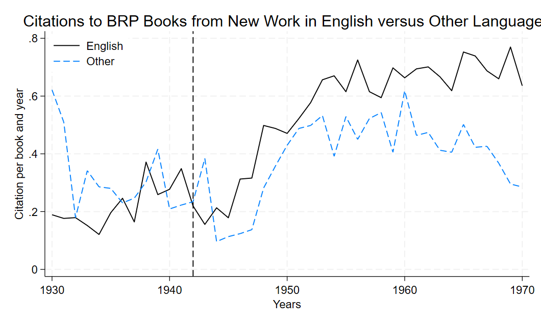
6.1.4 Figure 1 : Citations to BRP Books from New Work in English versus Other Languages

6.1.4.1 Preparation of the Data

In order to create the first figure, we need to prepare our data. In this step, we will demonstrate how to create a unique identifier and reshape the data from a wide format to a long format.

We have two variables representing the number of citations for each book, separated by whether the citations are from English-speaking authors count_eng or non-English-speaking authors count_noeng. Our goal is to consolidate this information into a single variable that reflects the total number of citations per book per year, along with a dummy variable English indicating whether the citation came from English-speaking authors or not. To achieve this, we generate two new variables: count1 for citations from English authors and count0 for citations from non-English authors. These are computed by subtracting the count_eng from the total number of citations.

We then use fakeid as an identifier to reshape our data from wide format to long format. Here, we encounter that the data is in a “wide” format where multiple observations are spread across columns rather than rows. To reshape this data into a more useful form, we introduce a unique identifier, fakeid which combines the id (book identifier) and year_c (year of citation). This fakeid ensures that we track each book’s data across years, allowing us to group observations correctly.

Reshaping the data from wide to long format is then necessary to combine related observations into a single record, that’s why we run the reshape long command, with i(fakeid) specifying the unique identifier and j(english) indicating the variable that identifies whether the citation came from English (count_eng) or non-English (count_noeng) author, once the two variable english and count created you can label them.

gen count1 = count_eng
gen count0 = cit_year - count_eng
replace count0 = 0 if count0 < 0 //ensure that there are no negative values

egen fakeid = group(id year_c)

reshape long count, i(fakeid) j(english) 

egen field_gr = group(field)

label var english "English"
label var count "count of citations"

6.1.4.2 Replication of the figure

the following code is being used:

The sort command organizes the dataset by the variable year_c (the year of citation). Sorting ensures that the data is in chronological order. This step is important for visualizing the data because graphs rely on properly ordered time series to make sense. And to saves a temporary version of the dataset, preserve helps us in changing the data. Any changes made after this point won’t affect the original data. And later, we can use the restore command get back the initial dataset. To create this graph,we’re interested in years after 1929, when the reform is being established, and that have citations to BRP Books . Thus, We filter the data keeping only rows where the year is later than 1929 by keep if year_c > 1929 that helps in doing this step. Then we drop if brp == 0 to remove rows where brp (Book Republication Program indicator) equals 0, focusing only on data related to books affected by the BRP.

The collapse (mean) command aggregates the data by averaging the variable count for each combination of year_c, english and post (whether the citation occurred after the BRP). This step simplifies the dataset by condensing it into one row per combination of these variables, making it easier to analyze and plot trends over time.

The graph is created using the twoway command, to plot two lines. One solid black line of medium width representing citation counts for English-speaking authors (if english == 1), the second line is blue , dashed and of medium width (lcolor(black) lpattern(dash) lwidth(medium)), it represents citation counts for non-English-speaking authors (if english == 0). A vertical dashed line is added at the year 1942 with xline, showing the year of the reform, the start of the BRP. The legend clearly distinguishes the two lines, with labels “English” and “Other,” positioned in the top-right corner without an outer ring legend(order(1 "English" 2 "Other") pos(11) ring(0)).

Once you have indicated all elements to draw in the twoway graph, you can customize it by adding a comma after each variable and write the design options (style, pattern and color of the line).then another comma and put the options of the graph: its title, y and x-axis titles, legend settings, and width. For example: The y-axis features here labels from 0 to 0.8 in intervals of 0.2 ylabel(0(0.2)0.8), while the x-axis features labels from 1930 to 1970 in intervals of 10 years which is put between the years(xlabel(1930(10)1970). Also, if you want to open and modify this graph later, graph save Saves the graph to the specified file path as a .gph file (Stata’s graph format).

Together, these customizations make the graph clear and informative, effectively visualizing the citation trends over time for English-speaking and non-English-speaking authors. Finally, we can restore our dataset that is not restricted to >1929 and can have brp that are equal 0.

sort year_c  
preserve 
keep if year_c >1929  
drop if brp == 0
collapse (mean) count, by(year_c english post)  
twoway (line count year_c if english == 1, lcolor(black) lpattern(solid) lwidth(medium)) (line count year_c if english == 0, lcolor(blue) lpattern(dash) lwidth(medium)), xline(1942, lcolor(black) lpattern(dash)) legend(order(1 "English" 2 "Other") pos(11) ring(0)) ytitle("Citation per book and year") xtitle("Years") ylabel(0(0.2)0.8) xlabel(1930(10)1970) title("Citations to BRP Books from New Work in English versus Other Languages")
graph save "Graph" "YOUR PATH.gph"
graph save "${Figs}/Graph1.gph", replace
restore

6.1.4.3 Output of the code

Graph 1

The graph shown above can be edited if you want to add a title or change the colors used you simply could click on data editor and then click edit once you finished save your changes and close the the graph editor simply by clicking on the icon. We changed here the color of the second line into blue.

This graph shows that before the BRP, counts of new publications that cite BRP books in English and other languages are similar in levels and trends and starts to deviate after 1942 when the BRP was implemented by Roosevelt, taking us back to the validation of the parallel trend assumption.

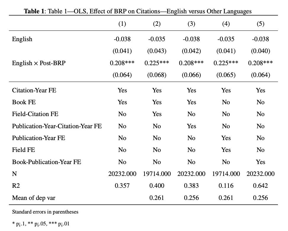
###Table 1: OLS, Effect of BRP on Citations—English versus Other Language

Table 1 is an OLS regression where the authors wanted to see the impact of BRP on citations of English versus other languages. We will learn here how to use different fixed effects and interactions between different fixed effects, and how to use local macros in our regressions. The following codes show how to do this.

6.1.4.4 The regressions

1. We will preserve so the changes will not affect the original dataset.

2. The c.english#c.post is used to do an interaction between those two variables. We clustered by id to take the correlation into account. The eststo stores the regression results into r1, that will be used in order to construct our final table with the different fixed effects.

3. In order to calculate the mean of the dependent variable, here count, for a subset of the sample, here for citations of English language authors before 1941, and to get the percentage increase in citations in response to BRP, we will store the results in r(mean) that is considered as a temporary macro. e(sample) is used to restrict the calculation to observations that were included in the regression above.

4. estadd is used to add a single value to the stored regression and scalar creates a new scalar named ymean in order that it is assigned the value of r(mean)

preserve 
keep if brp == 1 

//Column 1 

eststo r1: reghdfe count english c.english#c.post, absorb(id year_c) cluster (id) dof(none)  
qui sum count if e(sample) & year_c <= 1941 & english == 1
estadd scalar ymean = `r(mean)' 

5. If we don’t want to rewrite repeatedly the same regression with different fixed effects, we can define a local macro, for instance spec, which will save you time instead of rewrite the code over and over. To do so we will write the following codes :

local spec = "english c.english#c.post"

//Column 1 with fixed effects 

eststo r1: reghdfe count `spec', a(id year_c) cluster(id) dof(none)
estadd local citation_year_FE "Yes":r1
estadd local book_FE "Yes":r1
estadd local field_citation_FE "No":r1
estadd local pub_year_citation_year_FE "No":r1
estadd local publication_year_FE "No":r1
estadd local field_FE "No":r1
estadd local book_publication_year_FE "No":r1

estadd local ensures that the added statistic is temporary and tied to the current session. This is useful when you want to include specific information in your output without permanently altering the original estimation results.

6. We now are going to repeat what we have done for the first regression (column 1), but we will change now the fixed effects each time to account for the variations of different combinations. We used in the second regression i. instead of c. to create the interaction because they are categorical variables. Here, the interaction models the combined effect of the year and field categories. They used those fixed effects to capture the variation across fields over time.

//Column 2 

eststo r2: reghdfe count `spec', a(id year_c i.field_gr#i.year_c) cluster(id) dof(none)
qui sum count if e(sample) & year_c <= 1941 & english == 1
estadd scalar ymean = `r(mean)'
estadd local citation_year_FE "Yes":r2
estadd local book_FE "Yes":r2
estadd local field_citation_FE "Yes":r2
estadd local pub_year_citation_year_FE "No":r2
estadd local publication_year_FE "No":r2
estadd local field_FE "No":r2
estadd local book_publication_year_FE "No":r2


//Column 3 : FE control for the variation in citations across the life cycle of a book

eststo r3: reghdfe count `spec', a(id year_c i.publ_year#i.year_c) cluster(id) dof(none) 
qui sum count if e(sample) & year_c <= 1941 & english == 1
estadd scalar ymean = `r(mean)'
estadd local citation_year_FE "Yes":r3
estadd local book_FE "Yes":r3
estadd local field_citation_FE "No":r3
estadd local pub_year_citation_year_FE "Yes":r3
estadd local publication_year_FE "No":r3
estadd local field_FE "No":r3
estadd local book_publication_year_FE "No":r3

//Column 4

eststo r4: reghdfe count `spec', a(field_gr publ_year year_c) cluster(id) dof(none)
qui sum count if e(sample) & year_c <= 1941 & english == 1
estadd scalar ymean = `r(mean)'
estadd local citation_year_FE "Yes":r4
estadd local book_FE "No":r4
estadd local field_citation_FE "No":r4
estadd local pub_year_citation_year_FE "No":r4
estadd local publication_year_FE "Yes":r4
estadd local field_FE "Yes":r4
estadd local book_publication_year_FE "No":r4

//Column 5

eststo r5: reghdfe count `spec', a(i.id#i.year_c) cluster(id) 
qui sum count if e(sample) & year_c <= 1941 & english == 1
estadd scalar ymean = `r(mean)'
estadd local citation_year_FE "Yes":r5
estadd local book_FE "No":r5
estadd local field_citation_FE "No":r5
estadd local pub_year_citation_year_FE "No":r5
estadd local publication_year_FE "No":r5
estadd local field_FE "No":r5
estadd local book_publication_year_FE "Yes":r5

6.1.4.5 Replication of the Table 1

Now that we have all the regressions stored from r1 to r5 and the rmean stored in ymean as well, it’s time to get the final table. We will use the esttab command to generate a table using the stored regressions.

esttab r1 r2 r3 r4 r5 using "${Tables}/table1.tex", replace /// 
$options drop(_cons) stat(citation_year_FE book_FE field_citation_FE pub_year_citation_year_FE publication_year_FE field_FE book_publication_year_FE N r2 ymean , fmt(0 3 3) ///
label( `"Citation-Year FE"' `"Book FE"' `"Field-Citation FE"' `"Publication-Year-Citation-Year FE"'`"Publication-Year FE"' `"Field FE"' `"Book-Publication-Year FE"'`"N"' `"R2"' `"Mean of dep var"')) ///
nomtitle booktabs nogaps title("Table 1—OLS, Effect of BRP on Citations—English versus Other Languages")

restore 

• using "${Tables}/table1.tex", replace saves the output as a Latex file at the ${Tables} path defined above and overwrites it if it exists we use
• $option as a global macro here to avoid rewriting the same options another time and save time (the global has been defined and explained above)
• drop(_const) : drop our constant in the table
• stat() : includes which statistics to display:
  • N : number of observations
  • r2 : R-squared
  • ymean : mean of the dependent variable
  • list of the fixed effects included in the five regressions
  • fmt(0 3 3): format for each statistic, i.e. the number of decimal places
    • 0 (integer) for N
    • 3 for r2 and ymean
• label : descriptive name used to make those statics readable
• nomtitle : deletes model titles (default is to display r1, r2, etc., as titles)
• booktabs : formats the table using the LaTeX booktabs style, which improves table appearance
• nogaps : removes extra spacing between rows in the table, making it more compact
• titles : adds a title.

The table shows that in column 1, the coefficient indicates that citations to BRP books increased by an additional 0.211 citations per book and year after 1941, column 2 shows that even when accounting for the variations across fields over time, English-language citations increase by 0.229 per book and year. Columns 3, 4 and 5 are showing the results with different sets of fixed effects.

Table 1

6.1.5 Table 2: OLS, Effect of BRP on English-Language Citations: BRP versus Swiss Books (Matched Sample)

Since it is a triple-difference, we will now explain the second identification strategy that will be afterwards combined with their first. Their second identification strategy relies on comparing after 1941 the English-language citations to BRP books with English-language citations to Swiss books that were not eligible to BRP. This identification is used to make sure that this increase in citations is not caused by post war investments in science made by the USA.

To create a comparable sample of Swiss books, the authors use the Mahalanobis propensity score matching. So, they matched each BRP book with a Swiss book in the same research field and with a comparable pre-BRP stock of non-English-language citations, which will be used to construct Table 2 . They used also an alternative method which is the synthetic control as a robustness check. We will be explaining it we will need a other do file to do it, now lets replicate table 2.

Table 2 looks a lot similar to Table 1 (in terms of code writing). We decided to include it because it might be helpful when carrying the Triple-differences table (Table 3).

1. Since here you want to calculate the impact for a subset of the sample mainly the books that have been matched with Swiss books by the Mahalanobis propensity score :

preserve
keep if english == 1 & matched == 1

The main regression is : \[cites_{it} = βBRP_i × post_t + book_i + τ_t + ε_{it}\]

So the local macro is, as shown below, an interaction between BRP variable and post variable.

local spec = " c.brp#c.post" 

2. The rest is just as shown in Table 1 :

//Column 1 

eststo r1: reghdfe count `spec', a(id year_c) cluster(id) dof(none)   
qui sum count if e(sample) & year_c <= 1941 & brp == 1
estadd scalar ymean = `r(mean)'
estadd local citation_year_FE "Yes":r1
estadd local book_FE "Yes":r1
estadd local field_citation_FE "No":r1
estadd local pub_year_citation_year_FE "No":r1
estadd local publication_year_FE "No":r1
estadd local field_FE "No":r1


//Column 2 : the interaction in the fixed effects captures the idiosyncratic variation in citaions accross fields over time

eststo r2: reghdfe count `spec', a(id i.field_gr#i.year_c) cluster(id) dof(none)  
qui sum count if e(sample) & year_c <= 1941 & brp == 1
estadd scalar ymean = `r(mean)'
estadd local citation_year_FE "No":r2
estadd local book_FE "Yes":r2
estadd local field_citation_FE "Yes":r2
estadd local pub_year_citation_year_FE "No":r2
estadd local publication_year_FE "No":r2
estadd local field_FE "No":r2


//Column 3 : the interaction in the fixed effects capture the idiosyncratic variation for a book's age, with an interaction for publication year × citation year fixed effects

eststo r3: reghdfe count `spec', a(id i.publ_year#i.year_c) cluster(id) dof(none) 
qui sum count if e(sample) & year_c <= 1941 & brp == 1
estadd scalar ymean = `r(mean)'
estadd local citation_year_FE "Yes":r3
estadd local book_FE "Yes":r3
estadd local field_citation_FE "No":r3
estadd local pub_year_citation_year_FE "Yes":r3
estadd local publication_year_FE "No":r3
estadd local field_FE "No":r3

//Column 4 

eststo r4: reghdfe count `spec', a(year_c i.field_gr i.publ_year) cluster(id) dof(none)
qui sum count if e(sample) & year_c <= 1941 & brp == 1
estadd scalar ymean = `r(mean)'
estadd local citation_year_FE "Yes":r4
estadd local book_FE "No":r4
estadd local field_citation_FE "No":r4
estadd local pub_year_citation_year_FE "No":r4
estadd local publication_year_FE "Yes":r4
estadd local field_FE "Yes":r4

//Table 

esttab r1 r2 r3 r4 using "${Tables}/table2.tex", replace $options drop(_cons) stat( citation_year_FE book_FE field_citation_FE pub_year_citation_year_FE publication_year_FE field_FE N r2 ymean , fmt(0 3 3) label( `"Citation-Year FE"' `"Book FE"' `"Field-Citation FE"' `"Publication-Year-Citation-Year FE"'`"Publication-Year FE"' `"Field FE"' `"N"' `"R2"' `"Mean of dep var"')) nomtitle booktabs nogaps title("Table 2—OLS, Effect of BRP on English-Language Citations: BRP versus Swiss Books")
restore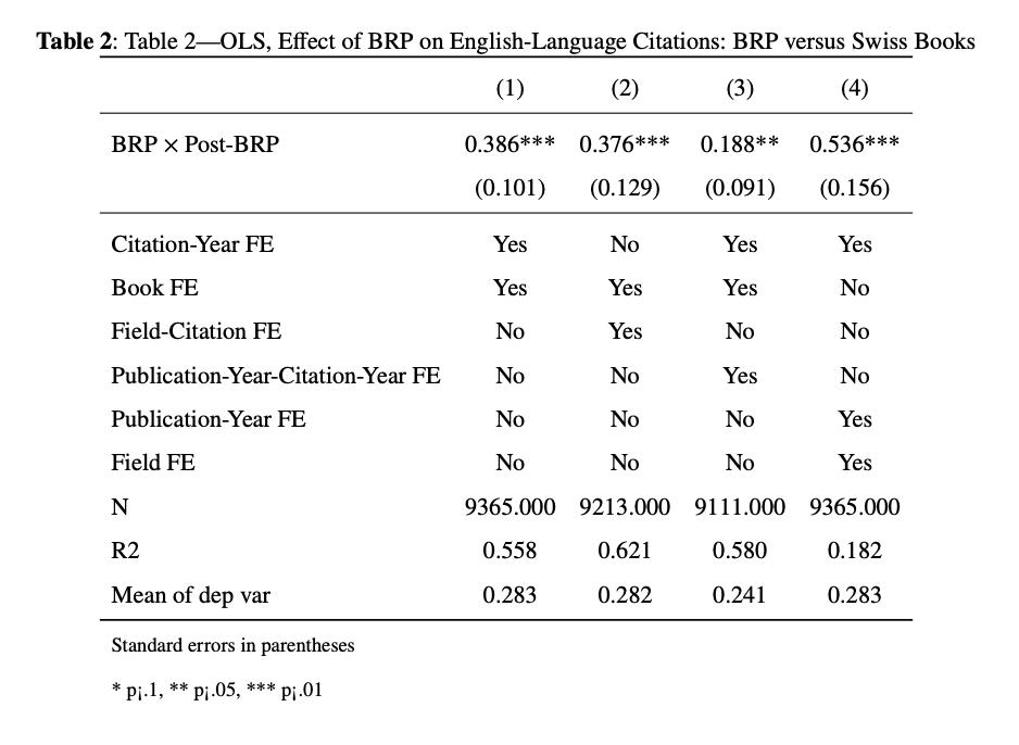 

Table 2

6.1.6 Table 3 : OLS, Effect of BRP on English-Language versus Other Citations: BRP versus Swiss Books (Matched Sample)

Now the regression changes to include the differential change in citations to BRP books from English-language and other-language authors with the same differential change for Swiss books. So here, there are 2 comparisons :

• the first examines changes in English-language citations to BRP books compared to citations to the same books in other languages, mitigating selection bias by focusing on the same source material across different linguistic contexts

• the second compares changes in English-language citations to BRP books with those to Swiss books, addressing the concern that English-language citations may have increased automatically due to a post-World War II. To account for this the authors are estimating the following equation :

\[cites_{ilt} = β_1English_l +β_2 BRP_i * post_t+ β_3 English_l * BRP_i + β_4 English_l * post_t+ β_5 English_l * BRP_i × post_t + book_i + τ_t + ε_{ilt}\]

where \(\beta_5\) is the coefficient of interest (the triple-difference coefficient). The local macro is defined accordingly and then, you repeat the steps of Table 1 and Table 2 with different specifications

preserve 
keep if matched == 1 
local spec = "english brp c.brp#c.post c.english#c.brp c.english#c.post c.english#c.brp#c.post" 

//Column 1

eststo r1: reghdfe count `spec', a(id year_c) cluster(id) dof(none) qui sum count if e(sample) & year_c <= 1941 & brp == 1 estadd scalar ymean =`r(mean)' estadd local citation_year_FE "Yes":r1 estadd local book_FE "Yes":r1 estadd local field_citation_FE "No":r1 estadd local pub_year_citation_year_FE "No":r1 estadd local book_citation_FE "No":r1 estadd local english_citation year "No":r1

//Column 2

eststo r2: reghdfe count `spec', a(id year_c i.field_gr#i.year_c) cluster(id) dof(none) qui sum count if e(sample) & year_c <= 1941 & brp == 1 estadd scalar ymean =`r(mean)' estadd local citation_year_FE "No":r2 estadd local book_FE "Yes":r2 estadd local field_citation_FE "Yes":r2 estadd local pub_year_citation_year_FE "No":r2 estadd local book_citation_FE "No":r2 estadd local english_citation year "No":r2

//Column 3

eststo r3: reghdfe count `spec', a(year_c i.field_gr i.publ_year) cluster(id) dof(none) qui sum count if e(sample) & year_c <= 1941 & brp == 1 estadd scalar ymean =`r(mean)' estadd local citation_year_FE "Yes":r3 estadd local book_FE "No":r3 estadd local field_citation_FE "No":r3 estadd local pub_year_citation_year_FE "Yes":r3 estadd local book_citation_FE "No":r3 estadd local english_citation year "No":r3

//Column 4

eststo r4: reghdfe count `spec', a(id year_c i.id#i.year_c) cluster(id) dof(none) qui sum count if e(sample) & year_c <= 1941 & brp == 1 estadd scalar ymean =`r(mean)' estadd local citation_year_FE "Yes":r4 estadd local book_FE "Yes":r4 estadd local field_citation_FE "No":r4 estadd local pub_year_citation_year_FE "No":r4 estadd local book_citation_FE "No":r4 estadd local english_citation year "Yes":r4

//Column 5 

eststo r5: reghdfe count `spec', a(id year_c i.english##i.year_c) cluster(id) dof(none) qui sum count if e(sample) & year_c <= 1941 & brp == 1 estadd scalar ymean =`r(mean)' estadd local citation_year_FE "Yes":r5 estadd local book_FE "No":r5 estadd local field_citation_FE "No":r5 estadd local pub_year_citation_year_FE "No":r5 estadd local book_citation_FE "Yes":r5 estadd local english_citation year "Yes":r5

//Table 

esttab r1 r2 r3 r4 r5 using "${Tables}/table3.tex", replace $options drop(_cons) stat(citation_year_FE book_FE field_citation_FE pub_year_citation_year_FE publication_year_FE field_FE N r2 ymean , fmt(0 3 3) label( `"Citation-Year FE"' `"Book FE"' `"Field-Citation FE"' `"Publication-Year-Citation-Year FE"'`"Publication-Year FE"' `"Field FE"' `"N"' `"R2"' `"Mean of dep var"' )) nomtitle booktabs nogaps title("Table 3—OLS, Effect of BRP on English-Language versus Other Citations: BRP versus Swiss Books")
restore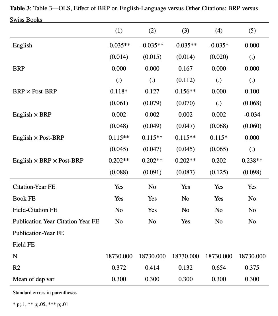

Table 3

6.1.7 Robustness checks: The Synthetic control Method

6.1.7.1 Synthetic dataset

In order to perform a synthetic control, we decided that we will use another do-file since this method is based on a lot of dataset generation and merging. We will then redefine our global macros and redownload our dataset:

clear
set more off
global Rawdata "C:YOUR PATH\raw data"
global Data "C:YOUR PATH\data"
global Figs "C:YOUR PATH\figs"
global Prog "C:YOUR PATH\prog"
global Tables "C:YOUR PATH\tables"
use "${Rawdata}/simplified_dataset.dta", clear 

To prepare a balanced dataset for performing the Synthetic Control Method (SCM), we start by filling any missing periods for the variable id to ensure the dataset is set as a balanced panel.

tsfill, full

Next, we assign integer values to each field, covering 25 mutually exclusive research fields within chemistry and 8 in mathematics, by grouping them into a new variable egen field_gr.

You can see through br command that most of the missing data points are in the early years. To handle this, we first sort the data by id in ascending and then by year putting a - sign before it to order it in descending order , ensuring that missing data points are placed at the end.

Remember the carryforward command being downloaded in the beginning ? We’ll use it now so that most recent available data is carried forward to fill the “early” missing years . So, for each id, the command will take the most recent (non-missing) values of field_gr, math, and publ_year and “carry” them forward to subsequent observations where those variables are missing using it to fill the gap.

For example, imagine a book’s field is recorded in 1950 but missing for 1948 and 1949. The command will take the value from 1950 and copy it backward to fill in the missing values for 1948 and 1949. This ensures that no data is left blank for earlier years and provides consistent information for analysis.

Afterward, the data is re-sorted by id and year in ascending order to arrange it chronologically.

The second bysort command aim to ensure that any remaining missing values in the variables (field_gr, math, and publ_year) are filled consistently, even after the initial use of carryforward After the carryforward process, any missing values . in the field_gr variable that still remain are explicitly replaced with 0, to ensure that no observations are left with missing values.

Finally, the dataset is restricted to keep years after 1920 to focus the analysis on the relevant period. These steps ensure the dataset is balanced and ready for SCM analysis.

tsfill, full
egen field_gr = group(field)
br
gsort id -year_c
bysort id: carryforward field_gr math publ_year, replace 
gsort id year_c

bysort id: carryforward field_gr math publ_year, replace
replace field_gr = 0 if field_gr == . 
keep if year_c > 1920

Now we are going to temporary save a subset of this the dataset that we will use later. Keeping only the 6 variables that are going to be included in the temporary dataset. id, year_c, brp count_eng , count_noeng cit_year, we sort them ascendingly, then we save this dataset that will be used then when constructing the synthetic control.

preserve
keep id year_c brp count_eng count_noeng cit_year
sort id year_c 
save temp.dta, replace  
restore

Now we are back to our original data set:

We keep only the variables used for conducting the synthetic control analysis, dropping the rest. Then, we rename the year_c variable to year for consistency.

Using tsset, we declare the dataset as a panel data set, using id as the panel identifier and year as the time variable, so it recognizes the repeated observations over time for each unit. It’s important to ensure once more that there are no missing values, as they will interfere with the synthetic control procedure, that’s why we use replace command. As before, sort the data by id in ascending order and by -year in descending order to correctly handle missing data points. Then creating different dummies for each research field using the gen(F) option with the tab command, generating frequency (tabulation) of the field_gr variable, creating a variable F that groups observations based on field categories.

keep cit_year count_eng count_noeng field_gr decl_perc id brp year_c math publ_year
rename year_c year
tsset id year
replace count_eng = 0 if count_eng == .
replace count_noeng = 0 if count_noeng == . 
gsort id -year
qui tab field_gr, gen(F)

It’s worth recalling that we are performing Synthetic controls procedure here in order to minimize pre-treatment differences between the treated unit (BRP) and the control unit. SCM does so by assigning different weights to the control variables.

Here we want to know how the outcomes specifically the number of English citations and non-English citations diverged after 1942 (the implementation date of BRP). We cannot simply compare Swiss and BRP books because they might differ in significant ways beyond the intervention that’s why the synthetic method is used, Stata has the synth package which we will be using (we already install it in the beginning). In order to use the synthetic method, we first determine our treatment and control groups for instance BRP is our treatment group and Swiss is our control group we have to declare the dataset as panel tsset and then we use the synth package.

Here, we will use levelsof command then we add our variable of interest, generating unique values of id, and our conditions (brp==1 and math==1) so its our treatment variable and we use local command that stores these unique id values into the local macro BRP for later use so it can loop over it. We do the same for the control group (Swiss). The conditions are made using if to ensure filtering only those groups that meet both criteria (brp == 1 and math == 1).

To create the loop, first, we use foreach command. this loop iterates over each group in the treatment group BRP and creates to each book its own synthetic control dataset, we use this brackets to begin and finish the loop {} We begin the loop using noisily command used to display messages or output without interrupting the flow of our code. Normally, disp (display) outputs text to the Results window, but if used directly, the code stops executing until the message is acknowledged. So, noisily allows you to display messages but ensures the code keeps running. Then you add the variable you want like this Book nr.'n' Inside the quotation marks, insert the current iteration value of n from the loop. For example, if n is 1, you’’ have: “Book nr. 1”.

Once declaring the data as a panel using tsset, we employ the synth command. The variables after it are the outcomes of interest, you make a comma and specify tour treatment units trunit('n') (each n from the BRP macro), identify your intervention year trperiod, specify the control variable the counit and finally, keep(book_n’, replace)` is used to create the new dataset. This code will keep running for a while.

Then you repeate the same steps for the chemistry fields’books where math == 0.

qui levelsof id if brp == 1 & math == 1, local(BRP)
qui levelsof id if brp == 0 & math == 1, local(Swiss)
foreach n of local BRP {
noisily disp "Book nr.'n'"
tsset id year
synth count_eng count_noeng, trunit('n') trperiod(1941) counit('Swiss') keep(book_'n', replace)
} 
qui levelsof id if brp == 1 & math == 0, local(BRP)
qui levelsof id if brp == 0 & math == 0, local(Swiss)
foreach n of local BRP {
noisily disp "Book nr. `n'"
tsset id year
synth count_eng count_noeng, trunit(`n') trperiod(1941) counit(`Swiss') keep(book_`n', replace)
}

We have our different synthetic datasets, and now we need to create our control group. First, we set obs 1 creating an empty observation, then gen x = . which adds a column x with missing values. This will create a temporary empty dataset called tempcontr.dta. This dataset will store the synthetic control group data for all treated books. For each treated book, we extract the corresponding control books and their synthetic control weights.

The merge command is then used to combine these control books’ data with the original dataset. After merging, we aggregate the data using the collapse command to compute synthetic control outcomes (count_eng, count_noeng, and cit_year) over time.

Finally, we append these synthetic control outcomes to the master control dataset (tempcontr.dta) and save the changes.It keeps iterating till we have all the synthetic control group.

For the other details in the code: qui levelsof id if brp == 1, local(BRP): it generates a list of unique IDs for books // here for both fields preserve: Saves the current state again for each treated book to restore after processing. clear: clears data to avoid interference from previous book’s data. use book_n'.dta: Loads the specific synthetic control dataset for book n. keep id weight: Keeps only the renamed variable id and weight to focus on control information. Sort the data by id to prepare for merging. merge 1:m id using temp.dta: Merges the control book data with the tempcontr.dta dataset by id. keep if _m == 3: Keeps only the matched observations, ensuring that the merge was successful. gen id_contr = n': Creates a new variable to label the synthetic control group for book n. collapse (mean) Aggregates the data, calculating the mean of outcomes //summarizes the control group’s data for the synthetic control comparison. gen brp = 0: Adds a brp indicator set to 0, distinguishing control units. save tempcontr.dta, replace: now we have our synthetic control group

preserve
clear
set obs 1
gen x = .
save tempcontr.dta, replace
restore
qui levelsof id if brp == 1, local(BRP) 
foreach n of local BRP {
preserve
clear
use book_`n'.dta
rename _Co_Number id
rename _W_Weight weight
keep id weight
sort id
merge 1:m id using temp.dta
keep if _m == 3   // only the matched results 
drop _m
drop id
gen id_contr = `n'
collapse (mean) count_eng count_noeng cit_year, by(id_contr year) 
gen brp = 0 
append using tempcontr.dta
save tempcontr.dta, replace 
restore
}

As a final step,we add everything in the same file

we first ensure that only the treated group(brp == 1). Next, we append the synthetic control group data stored in tempcontr.dta to the treated group. To avoid ID overlap between treated books and their synthetic controls, we add 50,000 to the IDs of synthetic control books, clearly distinguishing them from the treated group. We then create a linking variable that links each treated and control group for easier association between treated books and their respective synthetic control groups. To maintain consistency within each group, we calculate the maximum value of the math variable and the latest publication year (Year_from) for each group using egen. This ensures all books in a group are categorized consistently and have aligned publication years. Finally, we remove any observations where Year_from exceeds the analysis year (year), maintaining consistency across the treated and control groups.

`keep if brp == 1` 
`append using tempcontr.dta`
`replace id = id_contr + 50000 if brp == 0`
`replace id_contr = id if brp == 1`
bysort id_cont: egen Math = max(math)  
bysort id_cont: egen Year_from = max(publ_year) 
drop if Year_from > year 

6.1.7.2 Figure 2: Citations to BRP books and their synthetic controls

Here we’ll show how they constructed figureA13 in the appendix presenting the SC representation. Similar to figure 1, figure A13 is constructed the same way

`preserve`
collapse count_eng if year >= 1930, by(brp year)  
twoway  (line count year if brp == 1, lc(black)) (line count year if brp == 0, lp(dash) lc(black)), legend(order(1 "BRP" 2 "Synthetic controls")) xline(1942, lpattern(dash) lcolor(black)) ytitle("Citations per book and year")
graph save "Graph" "YOUR PATH\Graph2.gph"
restore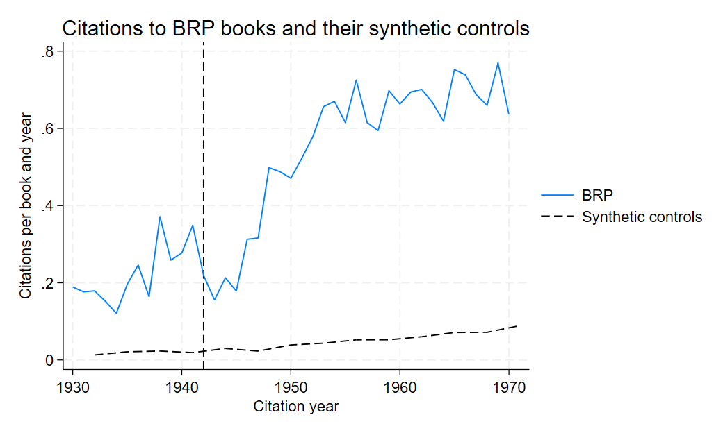

Graphe 2

The figure shows that the citation trends for BRP books diverge significantly from their synthetic controls following the key event (vertical line).This reinforces the main results, suggesting that the observed impact of the event on BRP books is not spurious and remains robust even when compared to a carefully constructed control group. Including this figure in the robustness checks confirms that the results are not sensitive to different specifications or methodological assumptions and strengthen the credibility of our analysis.

---

Authors: Salma Abdelsalam, Sara Sedrak, Mirana Ranerison, students in the Master program in Development Economics and Sustainable Development (2024-2025), Sorbonne School of Economics, Université Paris 1 Panthéon Sorbonne.

Date: December 2024