5.1 The Long-Term Effects of Measles Vaccination on Earnings and Employment

Atwood, Alicia. 2022. “The Long-Term Effects of Measles Vaccination on Earnings and Employment.” American Economic Journal: Economic Policy, 14 (2): 34–60. https://doi.org/10.1257/pol.20190509

Note: We used three datasets for our replication, as the author did since merging them was impossible. They are created and cleaned by the master do-file “0_master_do_cleaning.do”, which calls the three cleaning do-files for each dataset (“1_do_cleaning_inc_rate_ES.do”, “2_do_cleaning_results.do”, “3_do_cleaning_placebo_test.do”)

[Download 0_master_do_cleaning.do] [Download 1_do_cleaning_inc_rate_ES.do] [Download 2_do_cleaning_main_results.do] [Download 3_do_cleaning_placebo_test.do]

We then use these three datasets (“inc_rate_ES.dta”, “main_dataset_acs_200017.dta”, “placebo_dataset_acs196070.dta”) in the “4_dofile_results_LASCPE.do” to compute the tables and figure : [Download Do-File 4_dofile_results_LASCPE.do]

This is the codebook: [Download Codebook]

And the link to the replication package: [Link to the full original replication package paper from Open ICPSR]

Highlights

The article investigates the long-term effects of the measles vaccine on earnings and employment in the United States. Specifically, it examines how childhood exposure to the vaccine impacts adult labor market outcomes such as income, poverty, and employment rates.
It employs a staggered difference-in-differences (DiD) identification strategy. This approach exploits variation in pre-vaccination measles incidence rates across states and the staggered introduction of the vaccine, determined by birth cohorts and state-level differences in exposure timing.
The standard difference-in-differences method is commonly used in public health economics, as it captures the long-term benefits of improved health, such as better economic outcomes or reduction in the burden of disease.
This staggered DiD approach incorporate continuous treatment intensity, as pioneered by Bleakley (2007). It exploits geographic variation in pre-vaccination conditions, improving causal inference and capturing differential impacts across states and cohorts, in order to offer a more nuanced analysis of the vaccine’s long-term economic impacts.
Our added value relies mainly in the detailed explanation of the code for the original replication package, the creation of the code for Table 2 (as the authors do not provide it), and a discussion of new two-way fixed-effect estimators.
Stata tricks you will learn through this replication:
- How to generate an event-study graph with scatter plot.
- How to use a foreach command in order to loop over a list of dependent variables and store the corresponding results.
- How to create comprehensive results table with esttab.

5.1.1 Introduction

5.1.1.1 Paper Summary

In this paper, the author uses a staggered Difference-in-Differences (DiD) approach with continuous treatment to estimate the long-term impacts of measles vaccination on adult income and employment in the United States. The introduction of the measles vaccine in 1963 serves as a plausibly exogenous shock to childhood health. Leveraging geographic and temporal variations, the study measures exposure intensity through pre-vaccination measles incidence rates in an individual’s birth state.

Atwood (2022)’s paper reveals significant long-term economic benefits of measles vaccination on adult labor market outcomes, showing its crucial impact on individual and aggregate well-being:

Adults fully exposed to the vaccine, born in U.S. states with average pre-vaccine measles incidence rates, experience an increase in their annual income of $447 or 1.1% above the pre-vaccine cohort average. This income effect is even larger for those with non-zero incomes.
Beyond income, the vaccine reduces the likelihood of living in poverty by 0.5 percentage points. Employment likelihood also increases modestly by 0.29 percentage points, representing a 0.3% increase from the pre-vaccine cohort mean employment rate.
Notably, these gains can be attributed to productivity improvements rather than increased working hours, as average weekly hours slightly decline by 0.19 hours, a small but statistically significant result. On a national scale, these benefits translate into an estimated $76.4 billion annual increase in personal income in the U.S. (in 2019 USD), equivalent to 0.4% of total personal income.

Overall, these findings emphasize the economic potential of early childhood health interventions, i.e. vaccination, in reducing socio-economic inequalities. Robustness checks further validate the findings, demonstrating consistency across alternative sample restrictions and income segmentations.

5.1.1.2 Data

Data on Measles incidence rate. The data include annual state-level incidence rates for the population under 18, using (i) population estimates from Current Population Reports (CPS 1952–1968) and (ii) state-level case counts of particular diseases in the US published in the CDC’s Morbidity and Mortality Weekly Reports Annual Supplement (MMWR) from 1952 to 1975. These records cover measles, mumps, rubella, pertussis, and chicken pox, allowing analysis of disease trends pre- and post-vaccine availability. The measles vaccine was introduced in 1963. This dataset enables comparisons of health outcomes over time, highlighting the transformative effects of vaccination programs.

Data on Labor market outcomes. To measure labor market and income outcomes of individuals that were exposed to the disease and to the vaccine, the author uses the ACS (American Community Survey) database between 2000 and 2017, for individuals aged from 25 to 60 at the time of the survey. The sample is restricted to individuals born in the US, and for who it is possible to retrieve their state of birth. This allows the author to measure the exposure to measles and to the vaccine of individuals when they were children, avoiding issues related to selective migration.

5.1.1.3 Methodology

The Difference-in-Differences (DiD) method is a widely used econometric tool for estimating the effect of a treatment, such as a policy or program, by comparing outcome changes over time between a treatment group and a control group. In its classic form, DiD compares outcomes before and after a single intervention point for both groups. However, when treatment does not occur simultaneously across all units but is introduced at different times, a staggered Difference-in-Differences framework is employed. This framework accounts for the sequential rollout of interventions, allowing for more flexible modeling and increasing the number of possible comparisons.

The staggered DiD method exploits the varying timing of treatment adoption by comparing each treated group to others that have not yet received the treatment. This approach improves the reliability of causal estimates by incorporating temporal and spatial variation. Like the standard DiD method, it relies on the parallel trends assumption: outcomes for treated and untreated groups are assumed to follow the same trajectory in the absence of treatment. In the staggered case, this assumption applies to each group that receives treatment over time relative to others yet untreated.

In this paper, the author employs the staggered DiD framework to study the long-term effects of the introduction of the measles vaccine in 1963. This analysis draws on Bleakley (2007)’s methodology, which builds on the staggered approach by incorporating continuous treatment intensity and exploiting geographic variation in pre-intervention conditions to improve causal inference. Specifically, the study uses pre-vaccination measles incidence rates across states to measure treatment intensity and combines them with a staggered implementation of the vaccine across birth cohorts and states. By interacting state-level pre-vaccine measles incidence with birth-year-specific vaccine exposure, the author captures both the geographic and temporal dimensions of treatment variation. This continuous treatment intensity measure enhances the analysis, allowing for a detailed exploration of the vaccine’s long-term economic impacts. Bleakley (2007)’s approach is supposed to provide robust causal estimates by addressing confounders such as mean reversion and pre-existing trends.

5.1.1.4 Empirical Strategy

Aiming to isolate the causal impact of improved childhood health on adult economic outcomes, the empirical model draws upon staggered vaccine exposure, due to birth cohorts and state-level variations in pre-vaccine disease rates:

\[ Y_{isct} = \beta \left(M_{1952-1963}^{pre} \times \text{Exposure to Vaccine}_{sc}\right) + \delta_s + \gamma_c + \alpha_t + \theta X_{isct} + \epsilon_{isct} \]

focuses on measuring long-term effects of vaccine exposure on labor market outcomes, such as earnings or employment, for individual $i$ born in state $s$, from cohort $c$, and observed at year $t$. The key term $\left(M_{1952-1963, pre} \times \text{Exposure to Vaccine}_{sc}\right)$ captures the interaction between the pre-vaccine measles incidence rate $M_{1952-1963}^{pre}$ and the duration of an individual’s exposure to the vaccine. The $\beta$ coefficient estimates the differential impact of vaccine exposure across states with varying pre-vaccine measles incidence. Fixed effects $\delta_s, \gamma_c, \alpha_t$ account for state, cohort, and survey-year-level unobserved characteristics, while $X_{isct}$ controls for individual-level characteristics (such as gender and race).

The coefficient of interest $\beta$ relies on two sources of variation:

differential exposure of cohorts to the timing of the vaccine’s introduction
differential measles’ incidence rates across states.

Thus, $\beta$ gives the reduced-form estimate for the differences in labor market outcomes based on measles incidence rates before vaccine.

5.1.2 Good Practices Before Starting

5.1.2.1 Packages

To run this analysis you only need to install the estout package.

ssc install estout, replace

5.1.2.2 Folder Creation

Before starting the replication of this study, first create a structured folder system to organize your files and code efficiently.

Set up a main project folder and create 5 sub-folders within this one:

“raw_data”: Store here the datasets that are in the “raw_data” folder that you downloaded from the full original replication package.
“data_replication”. This is where we will store the cleaned datasets: “inc_rate_ES.dta” for the event-study graph, “main_dataset_acs_200017.dta” for the main results, and “placebo_dataset_acs_196070.dta” for the robustness check.
“do_files_replication”: you can store there the cleaning do-files and the do-file used in the rest of this replication (“4_dofile_results_LASCPE.do”).
“logs_replication”: this folder will store the log of the results. A log file is a record of everything that happens while you are using Stata, both what is written in the do-file and what Stata produces in response.
“output_replication”: this folder will contain the figure and tables you’ll create. Within this folder, create one sub folder named “tables” and another one named “figures”

In each do-file, the setting of globals (macro names that will help you store the paths to the folders as strings) is the following:

global home "~/replication_folder" //this is where you put the path to your main project folder

global tables           "$home/output_replication/tables"
global figures          "$home/output_replication/figures"
global do_files         "$home/do_files_replication"
global data             "$home/data_replication"
global raw              "$home/raw_data"
global logs             "$home/logs_replication"

5.1.2.3 Cleaning the data

In order to clean the data and to obtain the three datasets necessary to produce each one of the outputs, you first need to run the master do-file “0_master_do_cleaning.do”. This do-file is going to call each of the 3 cleaning do-files, in the right order, and is going to create three datasets in your “data_replication” folder.

Do not forget this step before trying to do the rest of the analysis!

5.1.3 Descriptive Statistics - Event Study

To identify the causal effect of vaccination on labor market outcomes and to validate the staggered DiD assumptions, the author first uses an event study analysis framework:

\[ Y_{ts} = M_{1952-1963}^{pre} \left[ \sum_{y=-6}^{-2} \alpha_y \mathbf{1}\{t - t^* = y\} + \sum_{y=0}^{11} \lambda_y \mathbf{1}\{t - t^* = y\} \right] + \delta_s + \gamma_t + \theta X_{ts} + \epsilon_{ts} \]

The above equation models the relationship between a dependent variable $Y_{ts}$ (e.g., the incidence of a disease) and the interaction of pre-vaccine measles rates $M_{1952-1963}^{pre}$ with event-time dummies. The terms $\mathbf{1}{t - t^* = y}$ capture event-time effects relative to the introduction of the measles vaccine, where $y$ indexes the years before or after the vaccine became available. The coefficients $\alpha_y$ represent pre-treatment trends, which are crucial for testing the parallel trends assumption of staggered DiD, while $\lambda_y$ estimate the impact of the intervention (vaccine availability) in post-treatment periods. The model includes state fixed effects $\delta_s$, year fixed effects $\gamma_t$, and covariates $X_{ts}$.

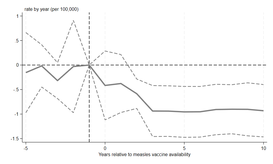
Figure 3: Event Study—Effect of Measles Vaccine on Measles Incidence

Figure 3 of the paper demonstrates the effect of the introduction of the vaccine on the incidence rate of measles.

We first load the primary dataset, “inc_rate_ES.dta”, which contains incidence rates for measles before and after the vaccine was introduced. Clearing existing data ensures no residual data interferes with our analysis:

use "$data/inc_rate_ES.dta", clear

To analyze the impact of pre-vaccine infection rates over time, we create interaction terms between yearly indicators (_Texp_i, i indicating the year) and the 12-year average measles rate per state (avg_12yr_measles_rate).

Specifically, we generate interaction terms for years 1 through 18, which capture pre-vaccine exposure rates. Note that year 6 is intentionally omitted as the reference year, anchoring the analysis and allowing for a comparative interpretation of effects across other years relative to this baseline.

local year "1 2 3 4 5 7 8 9 10 11 12 13 14 15 16 17 18"

foreach i of local year {
    gen exp_Mpre_`i' = _Texp_`i' * avg_12yr_measles_rate
}

Next, we run a regression analysis with measles incidence (Measles) as the dependent variable. The independent variables include the generated interaction terms (exp_M*), along with additional controls (state dummies, population size, exposure dummies). Then, the command cluster(statefip) ensures robust standard errors by accounting for correlation within states over time. This regression provides estimates of measles incidence both before and after vaccine introduction, adjusted for initial infection levels.

Finally, we use the regsave command to store the regression results, including confidence intervals and p-values. These results will be used later to facilitate the visualization of the event study findings through a graph.

reg Measles exp_M* _Is* population _T* avg_12yr_measles_rate,  cluster(statefip) robust

regsave, ci pval

For clarity in graphing, we modify the data to explicitly include a zero value for the omitted year (year 6) as the reference. Dropping unnecessary coefficients and setting all omitted values to zero ensure a consistent baseline for comparing effects in other years.

drop in 18/87

set obs 18
replace var = "exp_Mpre_6" in 18
replace coef = 0 in 18
replace stderr = 0 in 18
replace N = 1108 in 18
replace ci_lower = 0 in 18
replace ci_upper = 0 in 18

To establish a temporal structure for the interaction terms, we assign each interaction term a specific time point, relative to the vaccine’s introduction. Negative values indicate years before the vaccine, zero marks the year of vaccine introduction, and positive values represent years after. This time structure is essential for interpreting trends visually.

gen exp = .
foreach i in 1 2 3 4 5 6 7 8 9 10 11 12 13 14 15 16 17 18 {
    local value = `=`i'-7'
    replace exp = `value' if var == "exp_Mpre_`i'"
}
sort exp

The scatter command generates an event study graph plotting the coefficient estimates coef and confidence intervals ci* over time. Different line types and widths help differentiate the main estimates and confidence intervals, while yline(0) and xline(-1) mark reference points at zero and one year pre-vaccine, respectively. The x-axis shows years relative to vaccine availability, helping us interpret the effect timeline clearly.

scatter coef ci* exp if exp>-6 & exp<11,    c(l l l) cmissing(y n n) ///
                        msym(i i i) lcolor(gray gray gray) lpatter(solid dash dash) lwidth(thick medthick medthick) ///
                        yline(0, lcolor(black)) xline(-1, lcolor(black)) ///
                        subtitle("`sub' rate by year (per 100,000)", size(small) j(left) pos(11)) ylabel( , nogrid angle(horizontal) labsize(small)) ///
                        xtitle("Years relative to measles vaccine availability", size(small)) xlabel(-5(5)10, labsize(small)) ///
                        legend(off) ///
                        graphregion(color(white)) 
                    
                    
graph export "$figures/Figure3_event_study.png", replace

How to read Figure 3 ?

Figure 3 demonstrates that the common trend assumption is valid, as there are no statistically significant differences in measles incidence rates among states during the pre-vaccine period. After the introduction of the measles vaccine in 1963, marked by the vertical line in the figure, there is a sharp decline in measles incidence rates. This decrease is stabilizing approximately four years after the introduction of the measles vaccine, with a coefficient of $-1$. This coefficient indicates that for each unit of the pre-vaccine incidence rate, there was a one-for-one reduction in post-vaccine incidence, highlighting the vaccine’s effectiveness, especially in states with higher initial incidence rates.

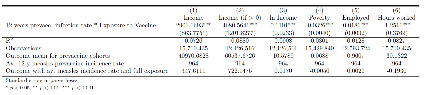
5.1.4 Main Results - TWFE

In order to obtain the main results of this paper, we will use the cleaned dataset of the American Community Survey (2000-2017), merged with measles rates data. To estimate the positive long-run effects of the measles vaccine on adults’ various outcomes (income, employment, poverty), the author uses a specification that allows for differential exposure to the measles vaccine, by interacting the measles rate pre-vaccine infection rate with a measure of the exposure to the vaccine, across states and cohorts of birth.

Table 2: Effects of Measles Vaccine on Adult Labor Market Outcomes

First, since our specification will include interaction terms, we drop interaction terms with empty cells. To explain this, let’s take a random example: if the variables “age” and “state of birth” are interacted, and you have no observations for two of your states, then the corresponding interaction outputs will be empty. Telling Stata to drop those terms will allow the code to run faster and will prevent errors.

set emptycells drop

Now, you are going to replicate the results of the table of main results, for every labor market and income outcomes.

This code will allow you to learn two techniques: - Using loops to run regressions, to avoid a repetitive process.

Using scalars in the estout package, to provide the complete table from Stata, with very little modification needed in LaTeX (or your preferred output format) to have a “publication style” table.

eststo clear

foreach dep in cpi_incwage cpi_incwage_no0 ln_cpi_income poverty100 employed hrs_worked {

    local controls i.bpl i.birthyr i.ageblackfemale i.bpl_black i.bpl_female i.bpl_black_female black female

    * Run main specification and store results
    reg `dep' M12_exp_rate `controls' i.year, robust cluster(bplcohort)
    eststo col`dep'
    
    *Add outcome means' line
    quietly summarize `dep' if exposure == 0
    local dep_mean = r(mean)
    estadd scalar dep_mean = `dep_mean'
    
    * Store the coefficient of M12_exp_rate
    scalar beta_`dep' = _b[M12_exp_rate]
    
    * Perform calculation with the stored coefficient
    scalar result_`dep' = beta_`dep' * (unweight_avg_12_measles_rate / 100000) * 16
    
    * Add scalars to the eststo model
    estadd scalar unweight_avg_12_measles_rate = unweight_avg_12_measles_rate
    estadd scalar calculated_result = result_`dep'
}

You are going to create a loop over the different dependent variables to run the main regression. This process is gonna take the following steps:

Start by creating a loop over all the dependent variables that are used in Table 2, and then, you can start working within the loop.
Since the controls are the same for each model, you can create a local with all the variables used as controls in this main specification.
Now, you can run a simple regression using the variable of interests, the local with controls, census year fixed effects and robust standard errors clustered at the state of birth by cohort level. Each iteration of the loop will then save the result of the regression for a different dependent variable with the command eststo, which we will then use to create the table.
You are now going to add rows 4 to 6 of Table 2, which are summary statistics and additional measures of the measles vaccine effect. First, you are going to calculate for each dependent variable its average for the prevaccine cohorts (i.e. those who were not exposed to the vaccine). Each mean is going to be stored in a scalar with the “estadd” function, which you will then display in the final table of results.
To obtain row 6 of the table of main results, the author says that she performed “back of the envelope calculations” to calculate the impact for each dependent variable of being born in a state with unweighted average prevaccine measles incidence rate (across all states) and full exposure to the vaccine. To do this, you need to perform this simple calculation in Stata: using the coefficient of interest (associated to the variable $measles\times exposure$) of each outcome variable, you need to multiply it by the unweighted average measles infection rate per 100,000 individuals, and then multiply this by 16 (number of years for full exposure).
Using estadd enables you to add to each iteration of the loop (and to each eststo col*) the scalars needed to replicate the rows 4 to 6 of the main results table: everything that you added with the estadd function is going to be stored along with the regression results for each dependent variable, under a different name.

After closing the loop, you can finally use the esttab function to replicate (almost) identically the main results table.

First, you are going to use each stored results under the prefix col*, and save them in a LaTeX format table in your output folder. The only coefficient you need to keep is the one associated with the variable of interest, and you can use the labels that you created before to display them in the table. To change the number of decimals for the coefficient and the standard errors, use b() and se().

In order to create rows 2 to 6, you can specify which “stats” you want in your table: here we want the R-squared, the number of observations and the different scalars that we stored earlier. fmt enables you to change the number of decimals you want to show, and you can modify the labels of each one of those stats. The code %9.0fc adds commas between thousands for numbers above 1,000 which is practical for readability.

esttab col* using "$tables/Table2_Main_results.tex", keep(M12_exp_rate) b(4) se(4) ///
label stats(r2 N dep_mean unweight_avg_12_measles_rate calculated_result, fmt(4 %9.0fc 4 0 4) ///
labels("R$^2$" "Observations" "Outcome mean for prevaccine cohorts" "Av. 12-y measles prevaccine incidence rate" "Outcome with av. measles incidence rate and full exposure")) replace

The results show a positive and significant effect of the vaccine on labor market outcomes across all specifications and measures of earnings. Indeed, the coefficient of row 6 in Column 3 can be interpreted as a 1.7 percent increase in income for an individual being born in a state with average measles incidence rate and full exposure to the vaccine.

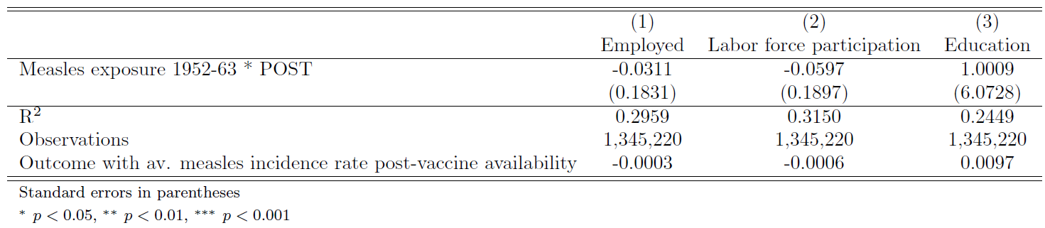
5.1.5 Robustness Check - Placebo Test

5.1.5.1 What is a Placebo Test ?

A placebo test is a method used to check if the results of a study are valid by applying the same analysis to a situation where no effect is expected. If no significant effect is found in the placebo test, it supports the reliability of the main results. However, if a significant effect appears, it suggests the findings might be influenced by errors, unaccounted factors, or random chance. This helps ensure the study’s findings are specific to the actual treatment or intervention.

5.1.5.2 In this case

The author conducts a test for contemporaneous effects by using adults aged 26 to 60 at the time of the 1960 and 1970 census. Since measles is a childhood illness, these individuals, who were already adults in 1963, would not have been eligible for the vaccine as they likely had measles in childhood. Therefore, the measles vaccine should have no impact on their immediate labor market outcomes.

To examine this, the Main Results equation is adjusted by interacting $M^{pre}_{1952-1963}$ with an indicator variable if the observation occurs after the measles vaccine has been introduced. The results show no statistically significant differences in employment, labor force participation, or years of education between adults in high-exposure and low-exposure states. These findings support the idea that the measles vaccine has short-term health impacts on the population it prevents from contracting measles, which in turn can lead to long-run impacts for those vaccinated.

Table 5: Contemporaneous Outcomes Check, Adult Labor Market Outcomes

5.1.5.3 Code explanation

To perform this placebo test, you will use the dataset containing contemporaneous labor market outcomes (placebo_dataset_acs196070.dta). The author examines the outcomes of adults during the vaccine introduction period to validate their TWFE methodology and assess the plausibility of the common trend assumption.

use "$data/placebo_dataset_acs196070.dta", clear

set emptycells drop

eststo clear

As in the Main Results section, begin by dropping interaction terms with empty cells. Then, clear the previously stored estimators to avoid conflicts when extracting the results table. The code structure will mirror that of the main results, employing a loop to run regressions for each dependent variable: employment status, labor force participation, and years of education.

The independent variable in these regressions is an interaction term between the pre-vaccine measles rate (1952–1963) and an indicator for whether the observation occurs after the introduction of the measles vaccine.

Within the loop, add a local macro to control for key variables, including sex, race, age, state, family income, and rural residency. The author uses a similar set of controls as in the main results to replicate the specification for a group of individuals who are unlikely to experience the vaccine’s positive effects.

To compute the estimated impacts of the regression coefficients, multiply each coefficient by the average measles incidence rate (0.00964). Note that the full exposure time (16 years) is not applied here, as the outcomes were measured before the full exposure period. A small discrepancy in point estimates for the calculated impact between our replication and the paper arises because the author expresses results in percentage points.

foreach dep in employed labforcepart edu_years2 {
    local controls i.year rural ruralpost female femalepost blackpost blackfemale   blackfemalepost i.age i.race i.statefip  famincome famincome2 famincome3

    reg `dep' M_post_rate_scale `controls' , cluster(statefip)
    eststo col`dep'
    
    * Store the coefficient of M_post_rate_scale
    scalar beta_`dep' = _b[M_post_rate_scale]
    
    * Perform calculation with the stored coefficient
    scalar result_`dep' = beta_`dep' * (unweight_avg_12_measles_rate / 100000) 
    
    * Add scalars to the eststo model
    estadd scalar calculated_result = result_`dep'
    }

Use the esttab command again to generate a self-contained table in LaTeX format. You can use the same options as in the main results section.

esttab col* using "$tables/Table5_placebo.tex", keep(M_post_rate_scale) b(4) se(4)  ///
label stats(r2 N calculated_result, fmt(4 %9.0fc 4) ///
labels("R$^2$" "Observations""Outcome with av. measles incidence rate post-vaccine availability")) replace

The results align with the author’s assumptions: the coefficients are statistically insignificant, and the calculated impacts are close to zero across all specifications. This supports the hypothesis that the measles vaccine had immediate effects on measles incidence and long-term labor market impacts for adults exposed to the vaccine as children.

5.1.6 Conclusion

In this study section, we have walked through the replication of “The Long-Term Effects of Measles Vaccination on Earnings and Employment” by Atwood (2022). We started by exploring the study’s research question and methodology, reviewing the staggered Difference-in-Differences (DiD) framework, and tackling advanced topics like continuous treatment intensity, event studies, and a placebo robustness check. Through this section, you can gain experience with important econometric tools and Stata coding skills, as used in academic research and policy evaluation.

5.1.6.1 Extension on new TWFE estimators

A limit of this paper is that it uses a two-way fixed effects estimator, with a staggered continuous treatment timing, as described in the Methodology section. However, as underlined by the Goodman-Bacon (2021). decomposition, the TWFE estimator is a weighted average of all $2\times2$ difference-in-differences estimators, and does not provide the causal effect of treatment on the outcome variable.

A solution to this caveat would be to use new TWFE estimators and compare the results with the specification used by the author. However, the Stata package necessary to implement new “clean” estimators does not yet exist for a continuous treatment (here, the measles incidence interacted with the length of exposure to the vaccine). Indeed, as showed by Callaway et al. (2024), the causal treatment effect can be identified on a generalized common trend assumption, in the way as previous estimators for binary treatments. However, it is not possible to interpret differences in the parameters across the different values of the continuous treatment (here, different measles incidence rates) as unbiased, due to selection on unobservables. They provide an alternative estimation strategy that do not suffer from these TWFE drawbacks, but the paper has yet no replication package to implement their new procedure.

For a more complete review of the (fast moving) literature on TWFE methods, we suggest you to look at Roth et al. (2023).

5.1.7 References

Atwood, Alicia. 2022. “The Long-Term Effects of Measles Vaccination on Earnings and Employment.” American Economic Journal: Economic Policy, 14 (2): 34–60. DOI: 10.1257/pol.20190509
Bleakley, H. (2007). Disease and Development: Evidence from Hookworm Eradication in the American South. The Quarterly Journal of Economics, 122(1), 73–117. http://www.jstor.org/stable/25098838
Callaway, B., Goodman-Bacon, A., & Sant’Anna, P. H. (2024). Difference-in-differences with a continuous treatment (No. w32117). National Bureau of Economic Research.
Goodman-Bacon, A. (2021). Difference-in-differences with variation in treatment timing. Journal of Econometrics, 225(2), 254-277. https://doi.org/10.1016/j.jeconom.2021.03.014
Roth, J., Sant’Anna, P. H., Bilinski, A., & Poe, J. (2023). What’s trending in difference-in-differences? A synthesis of the recent econometrics literature. Journal of Econometrics, 235(2), 2218-2244. https://doi.org/10.1016/j.jeconom.2023.03.008

Authors Elsa Poupelin, Camille Sirera, Anna Luntovska, students in the Master program in Development Economics (2024-2025), Sorbonne School of Economics, Université Paris 1 Panthéon Sorbonne.

Date December 2024