2.1 Winners and losers from Agrarian Reform: Evidence from Danish land inequality 1682–1895
Boberg-Fazlić, N., Lampe, M., Lasheras, P. M., & Sharp, P. (2022). Winners and losers from Agrarian Reform: Evidence from Danish land inequality 1682–1895. Journal of Development Economics, 155, 102813. https://doi.org/10.1016/j.jdeveco.2021.102813
[Link to the full original replication package paper on OSF]
Highlights
The paper examines the distributional effects of land reforms between 1682-1895 in Denmark.
The authors use an Instrumental Variable (IV) to deal with endogeneity issues stemming from reverse causality between the variable of interest (land productivity) and the dependent variable (land inequalities).
This methodology is standard by the choice of a geological instrument. It follows the usual steps of the IV procedure, including tests of the instrument’s pertinence (F-statistic of the 1st stage estimation).
Our added value to the original replication package lies mainly in the detailed explanation of the provided code. Additionally, we show how to extract various tables and figures directly from the Stata code.
We explain these Stata tricks:
Diagnostic Statistics: We leverage the
estat firststagecommand to obtain diagnostic statistics pertaining to the first-stage of instrumental variable estimation, which includes extracting and storing the F-statistics for further analysis.Looping: The
foreachloop structure is used, which enables the iteration over multiple years for instrumental variable regressions and allows to avoid repetitive commands in the code.Advanced Formatting: Through the utilization of the
esttabcommand along with various formatting options, we create well-formatted tables, which results in the production of tables that are not only clear and organized but also visually appealing.
2.1.1 Introduction
As a rule, agrarian reforms are viewed as fundamental for economic development, allowing, on one hand, to fuel agricultural productivity and on the other, to reallocate the necessary productive resources to industrialization. Their design has to fulfill two competing objectives: stimulating farms’ productivity and ensuring an equitable access to land. As numerous reforms have been criticized for failing the latter, this paper provides the first quantitative long-term assessment of the Danish agrarian reforms’ effects on both economic efficiency and land inequalities.
To do so, the authors combine several sources of historical data on farms at the parish level with population and agricultural censuses to cover the 1682-1895 period.
First, they document that the agrarian reform happened between 1784 and 1810, with a unification of property rights, favoring middle-sized farms.
Then, they get the number and sizes of farms per parish for the years 1682, 1834, 1850, 1860, 1873, 1885 and 1895 from Danish land registers, as well as their productive capacity measured in units of barrel of hard grain (HK), which was the unified measure used for tax collection.
Thanks to this data, they can calculate a measure for inequality within parishes for the several data points (their explained variable). They opt for the use of the Theil index to measure land inequality due to its analytically desirable properties. One key advantage is that the Theil index adheres to the principle of transfers, ensuring that a redistribution from one individual to a less affluent one results in a proportional decline in the Theil index, which is particularly convenient for focusing on changes in inequalities over time. Moreover, the Theil index provides unambiguous rankings of distributions, ensuring that two regions with identical Theil indices exhibit identical income distributions (not guaranteed by other common measures such as the Gini index). If a parish have all farms of equal productive size, then its Theil index is 0 ; if only one farm holds all land, its Theil index is the logarithm of the number of households living in the parish.
Finally, they consider the natural logarithm of the total value of the land (measured in HK) of parish p as their main explanatory variable.
Recall that their objective is to estimate the effect of productive capacity on inequality. From an econometric point of view, the most obvious approach would be to regress changes in parish-level land inequalities on a measure of soil productivity. Nonetheless, such a specification would be exposed to endogeneity issues, due to the reverse causality between the explained variable (evolution in land inequalities) and the variable of interest (land productivity): as higher agricultural productivity leads to Malthusian dynamics, in parishes with more fertile soils, there would be more smallholders and landless individuals, whose socio-economic status would then be deteriorated by the reforms. Consequently, areas with a higher agricultural productivity were more exposed to rises in land inequalities. At the same time, population growth has beneficial effects on innovation and thus, agricultural productivity. To tackle this, the authors adopt an IV strategy and choose as an instrument for land productivity the distribution of “Boulder Clay”, the sediment type most adapted to barley, resulting from the Weichselian glaciation. Geological variables are generally viewed as reliable instruments, since they capture long-term determinants of development that are independent from human factors. So their IV is the share of parish area classified as boulder clay (invariant in time).
2.1.2 Identification strategy
When deciding to use a 2SLS strategy, several points need to be discussed in order to allow the identification of robust causal effects. The first hypothesis to be considered and which cannot be tested statistically is the exclusion restriction. It is necessary to rule out any direct effect of the instrument (boulder-clay) on the dependent variable (land inequalities). In this specific case, it can be assumed that soil composition doesn’t directly affect the level of land inequalities. In fact, the authors argue that the rise of inequalities is driven by a stronger demographic growth, due to the productive capacity of the land. This implies, beside the soil fertility, adequate land management practices and efficient agricultural technologies. The authors also have to exclude any effect of the dependent variable on the instrument. Here, once again, land inequalities and the soil fertility seem to be unrelated, as the soil’s share of boulder clay stems from the Weichselian glaciation, which occurred approximately 18,000 years ago. Moreover, the sediment classification they use was made below the impact area of cultivation practices and technologies, which allows to infirm a potential effect of inequalities on this measure of land fertility.
The second hypothesis to be respected is the instrument’s relevance.
The authors need to convincingly describe how the instrument affects the
endogenous variable. In our case, the soil composition represents a key
determinant of the land’s productivity and thus is supposed to be
positively correlated with the total production of an area measured by
the variable TotalHK. Unlike the aforementioned exclusion restriction,
this assumption can be tested statistically. It can be done, for
instance, by verifying whether after estimating the first-stage
specification (1), the coefficient of the instrumental variable is
statistically significant or whether the F-statistic is superior to the
conventionally fixed value of 10.
\[\begin{equation} \tag{1} ln(TotalHK)_{p}=α_{0}+βBoulderClay_{p}+λ_{r}+X_{p}γ+ϵ_{p} \end{equation}\]
As we can see in column 2 of Table 1, the effect of the soil composition
on total production is statistically significant at 1% level. Also, the
value of the F-statistic is equal to 280. Hence, we can conclude that
both steps necessary to ensure the relevance and the exogeneity of the
instrument have been fulfilled. That said, they further estimate the
second-stage specification (2).
\[\begin{equation} \tag{2} ΔTheil_{p}=α_{0}+β\widehat{ln(TotalHK)}_{p}+λ_{r}+X_{p}γ+ϵ_{p} \end{equation}\]
After estimating both the OLS and the second-stage IV specifications, the authors find statistically significant positive effects of land productivity on land inequalities during the agrarian reforms. To ascertain the robustness of these findings, they estimate additional specifications, using alternative measures of land inequalities – such as Gini index, an alternative to the Theil index – and of land productivity – the amount of barley paid in tax. As no significant change in the results was detected, we can conclude that the econometric estimation allowed them to confirm their predictions, exposed in the theoretical part of the paper. In the next part of our narrative, we will discuss some of the main figures of the paper. We will also indicate the necessary commands to replicate them using Stata.
2.1.3 From the article to practice: exploring the replication code
2.1.3.1 Getting started: database access and required packages
In order to open the Stata database and execute the following lines of
code, several packages need to be downloaded and installed. In this
section, we guide you through the process of accessing the database and
briefly refer to these packages. In what follows, you have to download the original dataset from a link, then run these first lines of code to get the shorter version of the dataset, for which we also provide you with a codebook (see header).
***Open the database***
*download and save WinnersandLosers_finaldata.dta from: https://osf.io/jmn5y/files/osfstorage?view_only=f18f6d51efe44f04abef6e9042c0163c
*define your working directeory, where you also just stored the dataset
cd "C:\Users\" /*C:\Users\ = path where you also store the dataset*/

use "WinnersandLosers_finaldata.dta", clear
keep ID BygLG Lat Long year MLmean Theil_c AggTheil_c gini1682 gini1834 region ln_area LnDistCoast LnDistCPH ln_TotalFarmHK ln_Theil_1682c ln_Theil_1834c ln_Theil_1850c ln_Theil_1860c ln_Theil_1873c ln_Theil_1885c ln_Theil_1895c year_1 Gini ln_TotalFarmHK1682 ln_TotalFarmHK1834 ln_TotalFarmHK1850 ln_TotalFarmHK1860 ln_TotalFarmHK1873 ln_TotalFarmHK1885 ln_TotalFarmHK1895 ln_TotalFarmHK1682_nohouses ln_TotalFarmHK1834_nohouses ln_TotalFarmHK1850_nohouses ln_TotalFarmHK1860_nohouses ln_TotalFarmHK1873_nohouses ln_TotalFarmHK1885_nohouses ln_TotalFarmHK1895_nohouses
save "Dataset_AA_ALC_AT.dta", replace
Subsequently, several Stata packages are necessary to execute the
replication code successfully.
The first package needed is the estout package. This package allows
to make regression tables using regressions previously stored in the
Stata memory.
The second package required is the ivreg2 package. This package
allows to run instrumental variables regressions.
The third package is the coefplot package. This package is used to
create coefficients plots which visually represent the estimated
coefficients and their confidence intervals.
The fourth package is outreg2. This package is used to produce
illustrative tables of regression outputs. This package is able to write
LaTex-format tables.
All the packages can be installed using the following lines of code.
Table 1: IV estimation using total HK and the share of parish area classified as boulder clay
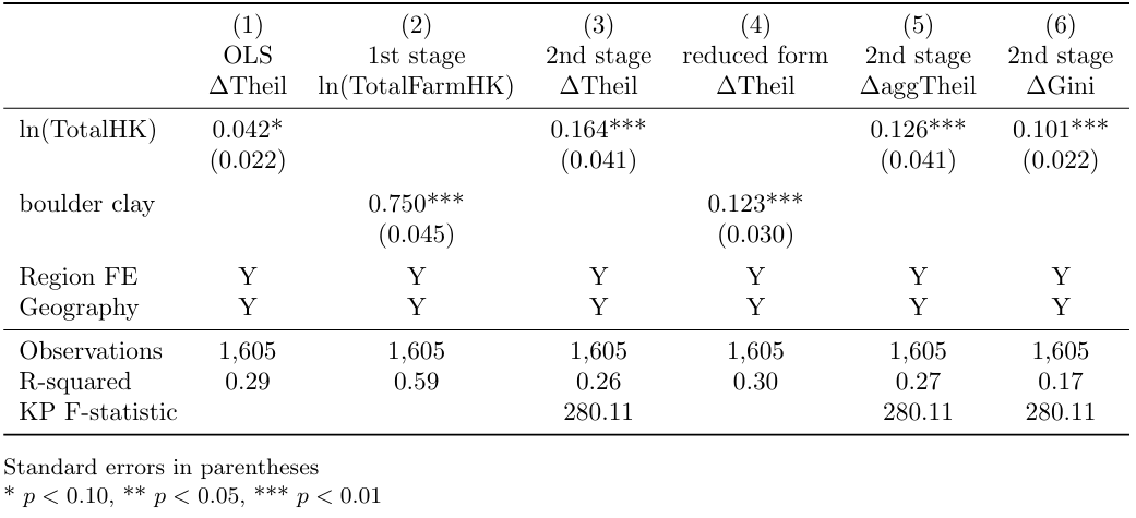
***Table 1***

use "Dataset_AA_ALC_AT.dta", clear

***Column (1) : OLS***
eststo ols1: qui reg D.Theil_c ln_TotalFarmHK ln_area LnDistCPH Lat Long LnDistCoast ///
  i.region if year==1834, vce(robust)

eststo ols2: qui reg D.AggTheil_c ln_TotalFarmHK ln_area LnDistCPH Lat Long LnDistCoast ///
  i.region i.year if year==1834, vce(robust)

***Column (2) : First-stage***
eststo fiv1: qui reg ln_TotalFarmHK MLmean ln_area LnDistCPH Lat Long LnDistCoast ///
  i.region if year==1834, vce(robust)

***Column (4) : Reduced form***
eststo ziv1: qui reg D.Theil_c MLmean ln_area LnDistCPH Lat Long LnDistCoast i.region ///
  if year==1834, vce(robust)

***Column (3) : Second-stage (with diffTheil)***
eststo ivdiff1: qui ivregress 2sls D.Theil_c ln_area LnDistCPH Lat Long LnDistCoast ///
  i.region (ln_TotalFarmHK = MLmean) if year==1834, vce(robust)
    estat firststage
    mat fstat = r(singleresults)
    estadd scalar Fstat = fstat[1,4]

***Column (5) : Second-stage (with diffAggTheil)***
eststo ivdiff2: qui ivregress 2sls D.AggTheil_c ln_area LnDistCPH Lat Long LnDistCoast ///
  i.region (ln_TotalFarmHK = MLmean) if year==1834, vce(robust)
    estat firststage
    mat fstat = r(singleresults)
    estadd scalar Fstat = fstat[1,4]

 ***Column (6) : Second-stage (with Gini)***
eststo ginihkdiff: qui ivregress 2sls D.Gini ln_area LnDistCPH Lat Long LnDistCoast ///
  i.region (ln_TotalFarmHK = MLmean) if year==1834, vce(robust)
    estat firststage
    mat fstat = r(singleresults)
    estadd scalar Fstat = fstat[1,4]

***Formation of Table 1***
esttab ols1 fiv1 ivdiff1 ziv1 ivdiff2 ginihkdiff, se star(* 0.10 ** 0.05 *** 0.01) b(3) ///
  r2 var(15) model(12) wrap keep(MLmean ln_TotalFarmHK) mtitles("OLS" "first stage" ///
  "second stage (diffTheil)" "reduced form (diff Theil)" "second stage (diffAggTheil)" ///
  "second stage (diffGini)" ) stats(N r2 Fstat, labels("Observations" "R-squared" ///
  "KP F-statistic") fmt(%9.0fc 2 2)) indicate("Region FE = 2.region" ///
  "Geography = LnDistCPH" , labels(Y N)) label
OLS regressions by replicating the columns 1,2 and 4 of Table 1
***Table 1***

eststo clear

***Column (1) : OLS***
eststo ols1: qui reg D.Theil_c ln_TotalFarmHK ln_area LnDistCPH Lat Long LnDistCoast ///
  i.region if year==1834, vce(robust)

eststo ols2: qui reg D.AggTheil_c ln_TotalFarmHK ln_area LnDistCPH Lat Long LnDistCoast ///
  i.region i.year if year==1834, vce(robust)

***Column (2) : First-stage***
eststo fiv1: qui reg ln_TotalFarmHK MLmean ln_area LnDistCPH Lat Long LnDistCoast ///
  i.region if year==1834, vce(robust)

***Column (4) : Reduced form***
eststo ziv1: qui reg D.Theil_c MLmean ln_area LnDistCPH Lat Long LnDistCoast i.region ///
  if year==1834, vce(robust)
Columns 1, 2, and 4 of Table 1 represent two Ordinary Least Squares
(OLS) regressions, a first-stage, and a reduced form, respectively,
representing distinct stages through OLS regressions. These different
model specifications are often used in econometric analyses to examine
causal relationships between variables. These columns offer a
comprehensive understanding of underlying economic relationships and
allow for nuanced interpretation of results. The singular variable
differing across the two OLS regressions is the initial variable,
corresponding to the dependent variable: the change in the Theil index
from 1682 to 1834 D.Theil_c and the change in the Theil index of
1834 aggregated to the size categories of 1682 D.AggTheil_c,
respectively. In line with our approach of conducting both the
first-stage and the reduced form analyses, we introduce the instrumental
variable MLmean in the two last regression equations. The
replication process of these columns involves several crucial steps in
estimating econometric models.
Firstly, the use of the eststo clear command ensures a reset of
previous estimation results, creating a clean environment before running
new estimations. Subsequently, the inclusion of qui – for quietly
– with the reg – for regress – function allows for the temporary
storage of regression results in a named matrix, such as ols1 in the
first model. Moreover, the model specification, denoted as
D.Theil_c ln_TotalFarmHK ln_area LnDistCPH Lat Long LnDistCoast i.region,
details the variables included in the regression equation. It is crucial
to note that this specification is essential for understanding the
relationships between key variables and the dependent variable – here
D.Theil_c or D.AggTheil_c. Furthermore, the use of the
conditional if year==1834 filters the data, retaining only
observations where the year variable is equal to 1834. This
filtering step enables a focus on a particular year – here 1834 –,
allowing for a more targeted analysis. Finally, the vce(robust)
option is specified to estimate robust standard errors, thereby
addressing potential heteroskedasticity issues. These robust standard
errors are particularly important to ensure the reliability of
estimation results, especially when residuals exhibit heterogeneous
variations.
IV regressions by replicating columns 3,5 and 6 of Table 1
***Table 1***

***Column (3) : Second-stage (with diffTheil)***
eststo ivdiff1: qui ivregress 2sls D.Theil_c ln_area LnDistCPH Lat Long LnDistCoast ///
  i.region (ln_TotalFarmHK = MLmean) if year==1834, vce(robust)
    estat firststage
    mat fstat = r(singleresults)
    estadd scalar Fstat = fstat[1,4]

***Column (5) : Second-stage (with diffAggTheil)***
eststo ivdiff2: qui ivregress 2sls D.AggTheil_c ln_area LnDistCPH Lat Long LnDistCoast ///
  i.region (ln_TotalFarmHK = MLmean) if year==1834, vce(robust)
    estat firststage
    mat fstat = r(singleresults)
    estadd scalar Fstat = fstat[1,4]

***Column (6) : Second-stage (with Gini)***
eststo ginihkdiff: qui ivregress 2sls D.Gini ln_area LnDistCPH Lat Long LnDistCoast ///
  i.region (ln_TotalFarmHK = MLmean) if year==1834, vce(robust)
    estat firststage
    mat fstat = r(singleresults)
    estadd scalar Fstat = fstat[1,4]
The columns 3, 5, and 6 which represent second-stages, are estimated
through instrumental variable regressions. Similar to OLS regressions,
the command eststo ivdiff1 : qui is used to store the estimation
results in a matrix named ivdiff1, ensuring an organized storage of
relevant information. Secondly, the function ivregress 2sls is
applied to conduct a two-stage IV regression, as indicated by 2sls.
Additionally, the explanatory variables
D.Theilc lnarea LnDistCPH Lat Long LnDistCoast i.region mirror those
used in the OLS regressions, providing continuity in the model
specification. The only variable differing across each column
specification is the initial variable, corresponding to the dependent
variable : the change in the Theil index from 1682 to 1834 D.Theilc,
the change in the Theil index of 1834 aggregated to the size categories
of 1682 D.AggTheilc, and the change in the Gini coefficient instead
of the Theil index D.Gini, respectively. This nuanced change
reflects the distinct focus on different dependent variables in each
instance, while the remaining explanatory variables remain constant,
allowing for a systematic exploration of the impact of the selected
variables on the varied dependent variables. The inclusion of
(lnTotalFarmHK = MLmean) specifies the endogenous variable
lnTotalFarmHK and its instrument MLmean. This crucial
specification distinguishes the endogenous variable and its
corresponding instrument, a fundamental aspect of instrumental variable
estimation. Furthermore, to address heteroskedasticity and
autocorrelation, the vce(robust) command employs a robust
variance-covariance matrix, ensuring the reliability of standard errors
in the estimation.
The upcoming lines of code that we are about to describe initially
seemed somewhat unclear to us. However, despite the initial ambiguity,
they prove to be valuable and, upon closer examination, are now better
understood. This is why we will take the time to provide a clear
explanation of these lines. First, the line estat firststage is
employed to display statistics from the first-stage of the IV
regression. This step is typically utilized to assess the validity of
instruments and ascertain their suitability for the estimation process.
Secondly, storing the first-stage results in a matrix named ‘fstat’ is
accomplished through the line mat fstat = r(singleresults). This
matrix captures relevant statistics from the first-stage, providing a
comprehensive view of the instrumental variable performance. Finally,
the line estadd scalar Fstat = fstat[1,4] introduces a new scalar
variable, Fstat, into the main regression results. This step allows
to extract the F-statistic from the first-stage matrix fstat and
assigns it to Fstat. The F-statistic is a crucial metric in
instrumental variable regression, serving as a diagnostic tool to assess
the overall validity of the instruments used. A high F-statistic, that
is superior to 10, suggests that the instruments collectively have a
strong explanatory power for the endogenous variable. In summary, these
lines of code are essential for evaluating the quality and relevance of
the instrumental variables employed in the two-stage IV regression.
Formatting Table 1, an additional but optional step
***Table 1***

***Formation of Table 1***
esttab ols1 fiv1 ivdiff1 ziv1 ivdiff2 ginihkdiff, se star(* 0.10 ** 0.05 *** 0.01) b(3) ///
  r2 var(15) model(12) wrap keep(MLmean ln_TotalFarmHK) mtitles("OLS" "first stage" ///
  "second stage (diffTheil)" "reduced form (diff Theil)" "second stage (diffAggTheil)" ///
  "second stage (diffGini)" ) stats(N r2 Fstat, labels("Observations" "R-squared" ///
  "KP F-statistic") fmt(%9.0fc 2 2)) indicate("Region FE = 2.region" ///
  "Geography = LnDistCPH" , labels(Y N)) label
The next stage in our analysis involves the creation of a comprehensive
table summarizing the results of the previously conducted regressions.
It is essential to note that this step does not stand alone, rather it
complements the preceding two steps in which variables were defined and
regressions were estimated. The resulting table serves as a visual
representation of the relationships captured in the regression models,
enhancing the interpretability and communicative power of the findings.
First, the command esttab ols1 fiv1 ivdiff1 ziv1 ivdiff2 ginihkdiff
specifies which models to include in the table, incorporating the
Ordinary Least Squares (OLS), first-stage instrumental variable (IV),
and second-stage IV regression results. To enhance the clarity of the
table, additional formatting options are applied. The
se star(* 0.10 ** 0.05 *** 0.01) command displays standard errors
with significance stars, denoting significance levels with asterisks.
Thirdly, the b(3) command allows to limit coefficient estimates to
three decimal places, contributing to a cleaner presentation of results.
Moreover, the inclusion of r2 displays the coefficient of
determination, the R-squared, in the table, providing insights about the
explanatory power of the model. The var(15) option limits the
display of R-squared to 15 decimal places.
Additionally, with model(12), we specify the maximum number of
models to display in the table, accommodating up to 12 different model
specifications. The wrap command facilitates the wrapping of long
variable names onto multiple lines, ensuring readability. The
keep(MLmean lnTotalFarmHK) option selectively includes only the
variables MLmean and lnTotalFarmHK in the table, which are our
instrument and endogenous variables. Furthermore, mtitles() assigns
model titles to each specified model, contributing to a more informative
and organized presentation. The
stats(N r2 Fstat, labels("Observations" "R-squared" "KP F-statistic") fmt(%9.0fc 2 2))
option adds relevant statistics to the table, including the number of
observations (N), the R-squared, and the F-statistic. The
indicate ("Region FE = 2.region" "Geography = LnDistCPH", labels(Y N))
command introduces indicator in a regression model. The first part,
"Region FE = 2.region", includes fixed effects for a specific
region, here denoted as 2, representing Jutland. This accounts for
unobserved variation specific to Jutland. The second part,
"Geography = LnDistCPH", introduces an indicator variable related to
geography. The labels Y and N are assigned to indicate the
presence or absence of fixed effects or controls in each observation,
contributing to the model’s interpretability. This step allows for a
nuanced interpretation of how fixed effects and geographic controls
influence the results. Finally, the label option is appended to the
esttab command, indicating that variable labels should be included
in the table for clarity and precision.
In the replication code provided by the authors, no specific instruction
regarding the exportation of tables has been included. Therefore, we
recommend users to add the command using "NameOfYourTable.tex" right
after the last variable mentioned in esttab, just before the comma
in front of se star, if they intend to export the table in LaTeX
format. Alternatively, users can use the command
using NameOfYourTable.txt", at the same location in the code, if
they prefer the table in a text format. This flexibility allows users to
choose the desired output format for the tables based on their specific
needs.
This last step – which involves the formation of the table – can be
used in the context of other studies to generate a clear and visually
appealing table summarizing regression results. However, it is crucial
to emphasize that this step is not indispensable for obtaining
replication results. The results can be independently observed directly
using the same code without the qui option, starting from reg or
ivreg. This underscores the flexibility of the code, allowing
researchers to directly access and analyze the regression outcomes
without relying on the table generation step. While the table
contributes to a more organized presentation, it is not a prerequisite
for the replication process. Users can tailor their analysis based on
their preferences and requirements before proceeding to this step. The
study relies on an instrumental variable method that can be challenging
to comprehend. Explaining the replication code of Table 1 is deemed
essential for us, as it allows a detailed exploration and validation of
the authors’ instrumental variable approach. This importance is further
underscored by the fact that Table 1 showcases the primary results of
the study. Having elucidated the intricacies of the Table 1 replication
code, we will now transition to describing the replication code for
Figure 5.
Figure 5
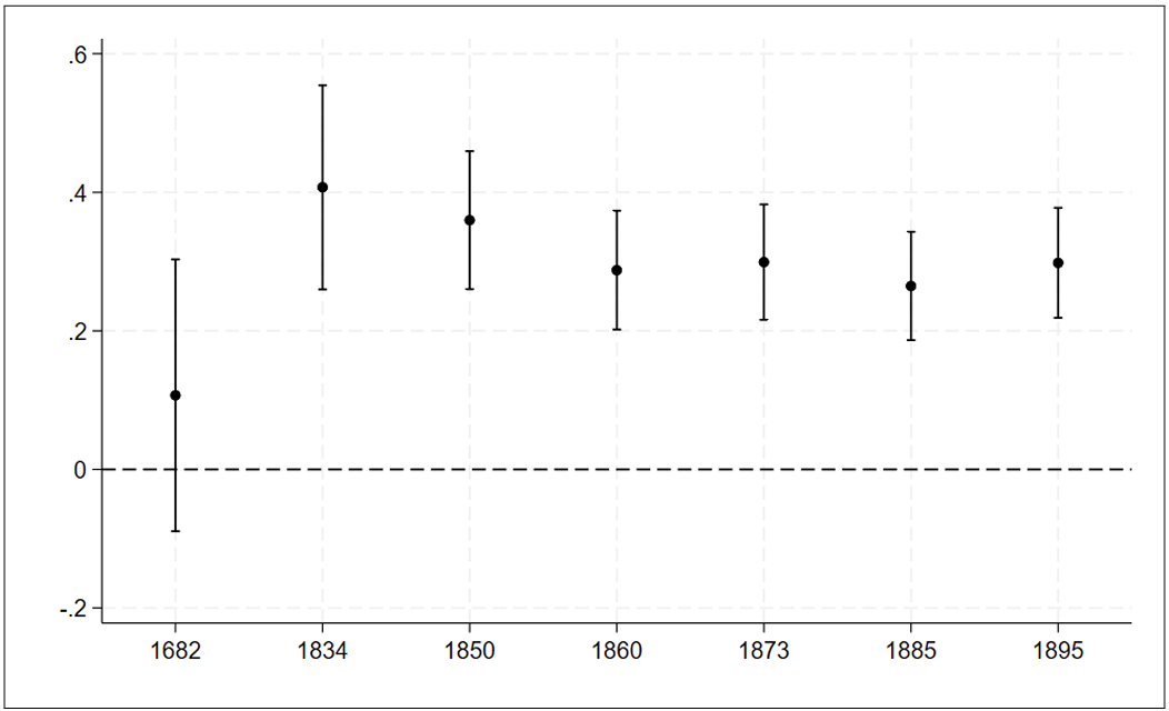
***Figure 5***

eststo clear

foreach x in 1682 1834 1850 1860 1873 1885 1895 {
    qui ivregress 2sls ln_Theil_`x'c ln_area LnDistCPH Lat Long LnDistCoast i.region ///
      (ln_TotalFarmHK`x' = MLmean) if year==`x', vce(clust ID)
    estimates store coef`x'
}
    coefplot coef*, vert yline(0) keep(ln_TotalFarmHK*) graphregion(color(white)) ///
      ciopts(recast(rcap) lcol(black)) mcolor(black) xtick(1(1)7) ///
      xlabel(1 "1682" 2 "1834" 3 "1850" 4 "1860" 5 "1873" 6 "1885" 7 "1895", ) ///
      grid(b) legend(off)
graph export "outputfile.png", replace
The provided Stata code segment serves to illustrate the coefficients
for second-stage estimations conducted over the years 1682 to 1895. The
dependent variable under consideration is ln(Theil), and the
instrumental variable utilized is the share of boulder clay MLmean.
The use of the natural logarithm for the dependent variable
ln(Theil) in the second-stage regression is intentional. This choice
allows for the presentation of estimates for the second-stage
coefficients in levels, offering insight into the relationships over the
years 1682 to 1895. The focus on ln(Theil) in different years
underscores a preference for examining the absolute values of Theil
index rather than changes in Theil index, providing a comprehensive
perspective on the dynamics of the variable across the specified
temporal range.
Initially, eststo clear ensures a clean slate by clearing any
previously stored estimation results. Subsequently, the foreach loop
in the provided Stata code serves as an iterative mechanism, allowing
the execution of specified commands for each value in the specified
range or list. In this case, the loop iterates over the years 1682,
1834, 1850, 1860, 1873, 1885, and 1895. For each iteration, the code
within the loop conducts a 2-stage least squares regression using the
ivregress 2sls command, estimating a model for the given year. The
model includes various independent variables such as
lnTheil’x’c, lnarea, LnDistCPH, Lat, Long, LnDistCoast as
well as the endogenous variable lnTotalFarmHK instrumented by
MLmean and there are fixed effects for region. The purpose of
the loop in this context is to efficiently run the same regression model
for multiple years, automating the process and avoiding redundant code.
This is particularly useful when dealing with time-series data or when
conducting analyses for various time points. The resulting coefficient
plot provides a concise and visual representation of the dynamics of the
variable of interest across different years. The line
estimates store coef’x’ facilitates the storage of estimation
results in matrices named coef’x’, where x represents the
specific year. Following the loop, the coefplot coef* command
generates a coefficient plot based on the stored estimation results,
specifically focusing on coefficients related to the variable
lnTotalFarmHK across the years.
In terms of visual representation, the plot includes a vertical line at
0 for reference with the vert yline(0) command, retains only
coefficients related to lnTotalFarmHK with the
keep(lnTotalFarmHK*) command, and employs a white background for
enhanced clarity thanks to the graphregion(color(white)). Confidence
intervals are displayed using a horizontal line in black with
ciopts(recast(rcap) lcol(black)), and the markers – dots –
representing coefficient estimates are colored black for visibility with
the mcolor(black) option. Additionally, xtick(1(1)7) and
xlabel(1 "1682" 2 "1834" 3 "1850" 4 "1860" 5 "1873" 6 "1885" 7 "1895"),
allow stick marks and corresponding labels on the x-axis to be
strategically positioned to represent each year from 1682 to 1895.
Gridlines are incorporated for ease of interpretation grid(b), and
the legend is turned off for a clean and uncluttered visual
representation thanks to the legend(off) command.
The final line of code, graph export "outputfile.png", replace, is
added by us to the replication code for the purpose of exporting the
coefficient plot as a PNG file. This command utilizes Stata’s graph
export feature, allowing us to save the generated graph to an external
file named “outputfile.png” in the current working directory. The
option "replace" ensures that if a file with the same name already
exists, it will be overwritten. This line of code enhances the
replicability of the study by facilitating the export of the coefficient
plot in a widely used PNG format for further analysis or inclusion in
reports and presentations. This meticulous approach allows for a
comprehensive exploration of coefficient dynamics over time, offering
insights into the relationship between the dependent variable,
ln(Theil), and the instrumental variable MLmean – share of
boulder clay – with controls included, across the specified years. With
the explanation of the coefficient plots for second-stage estimations
complete, our attention now shifts to describing the replication code
for Table A.3 found in the Appendix.
Table 3: Robustness check: Second-stage IV estimates using Gini coefficient

***Table A.3***

***Creation of a loop***
eststo clear
foreach x in 1682 1834 {
    eststo ginihk`x': ivregress 2sls gini`x' ln_area LnDistCPH Lat Long LnDistCoast ///
      i.region (ln_TotalFarmHK = MLmean) if year==`x' & gini1834!=., vce(clust ID)
    estat firststage
    mat fstat = r(singleresults)
    estadd scalar Fstat = fstat[1,4]
}

***Formation of Table A.3***
esttab ginihk1682 ginihk1834, se star(* 0.10 ** 0.05 *** 0.01) b(3) r2 var(15) model(11) ///
  wrap keep(ln_TotalFarmHK) mtitles("2nd stage: Gini diff" "2nd stage: gini 1682" ///
  "2nd stage: gini 1834") stats(N r2 Fstat, labels("Observations" "R-squared" ///
  "KP F-statistic") fmt(%9.0fc 2 2)) indicate("Region FE = 2.region" ///
  "Geography = LnDistCPH" , labels(Y N)) label
Table A.3 in the Appendix presents robustness check results, specifically second-stage instrumental variable estimates using the Gini coefficient. This additional analysis aims to verify the robustness of the findings by employing an alternative measure. The choice of the Gini coefficient not only enhances interpretability but also provides a basis for comparing and validating the study’s results against a broader scholarly context.
Creation of a loop
***Table A.3***

***Creation of a loop***
eststo clear
foreach x in 1682 1834 {
    eststo ginihk`x': ivregress 2sls gini`x' ln_area LnDistCPH Lat Long LnDistCoast ///
      i.region (ln_TotalFarmHK = MLmean) if year==`x' & gini1834!=., vce(clust ID)
    estat firststage
    mat fstat = r(singleresults)
    estadd scalar Fstat = fstat[1,4]
}
Firstly, the use of the eststo clear command ensures a reset of
previous estimation results, creating a clean environment before running
new estimations. The loop designated by foreach x in 1682 1834
iterates over two specific years, namely 1682 and 1834. This looping
mechanism, as explained in the preceding section – Section 3.3 –,
provides a concise and efficient way to conduct repetitive tasks for
multiple years. The eststo ginihk‘x’ command within the loop
facilitates the storage of results in matrices named ginihk‘x’, with
x representing the current year in each iteration. For a more
comprehensive understanding of the loop creation and its purpose,
referring to the preceding Section 3.3 is recommended. Moreover, the
ivregress 2sls function is employed to conduct a two-stage
instrumental variable (IV) regression. The model’s explanatory variables
include D.Theil_c ln_area LnDistCPH Lat Long LnDistCoast i.region.
In specifying (ln_TotalFarmHK = MLmean), the endogenous variable –
the natural logarithm of the total value of the land measured in barrel
of hard grain of parish – is denoted as ln_TotalFarmHK and its
instrument is identified as MLmean.
To ensure that the analysis includes only observations for the specified
year x where the variable gini1834 is not missing, the condition
if year==x & gini1834!=. is incorporated. Furthermore, the command
vce(clust ID) is used to adjust standard errors in the regression
model, accounting for within-cluster correlation. The code that we will
now describe mirrors the structure found in Table 1. Following this,
estat firststage is employed to display statistics from the
first-stage of the IV regression. This step is crucial for assessing the
validity of instruments. The subsequent lines involve the storage of
first-stage results in a matrix named fstat using the
mat fstat = r(singleresults) command. This matrix captures relevant
statistics from the initial stage, providing insights into the
instrumental variable performance. Finally,
estadd scalar Fstat = fstat[1,4] introduces a new scalar variable
Fstat into the main regression results. This step extracts the
F-statistic from the first-stage matrix fstat and assigns it to
Fstat. For a more comprehensive understanding of the F-statistics
and its purpose, referring to the preceding Section 3.3.2 is
recommended.
Formatting table A.3, an additional but optional step
***Table A.3***

***Formation of Table A.3***
esttab ginihk1682 ginihk1834, se star(* 0.10 ** 0.05 *** 0.01) b(3) r2 var(15) model(11) ///
  wrap keep(ln_TotalFarmHK) mtitles("2nd stage: Gini diff" "2nd stage: gini 1682" ///
  "2nd stage: gini 1834") stats(N r2 Fstat, labels("Observations" "R-squared" ///
  "KP F-statistic") fmt(%9.0fc 2 2)) indicate("Region FE = 2.region" ///
  "Geography = LnDistCPH" , labels(Y N)) label
Moving forward in our analysis, we proceed to construct a comprehensive
table that consolidates the outcomes of the earlier regression analyses.
Importantly, it’s crucial to emphasize that this stage is not conducted
in isolation, instead it builds upon the groundwork laid in the
preceding step where variables were defined and regressions within the
loop were executed. The resultant table serves as a visual
representation, effectively summarizing the relationships captured in
the regression models. This approach enhances the interpretability and
communicative power of the analytical findings. The code employed in the
creation of the comprehensive table A.3 aligns with the methodology
elucidated in Section 3.2.3, specifically used for Table 1. Indeed, the
Stata code provided encompasses the construction of a table using the
esttab command, incorporating results from the two-stage
instrumental variable regressions conducted for the years 1682 and 1834.
Thus, the esttab ginihk1682 ginihk1834 line specifies the models
whose results will be included in the table, representing these two
specific years.
To enhance the clarity and readability of the table, several formatting
commands are employed. The se star(* 0.10 ** 0.05 *** 0.01) line
introduces significance stars denoted by asterisks, indicating the
levels of statistical significance. Additionally, b(3) limits the
coefficient estimates to three decimal places. The inclusion of the
coefficient of determination R-squared is facilitated by r2 command,
with var(15) limiting the number of decimals for R-squared to 15
digits. The model(11) command specifies the maximum number of models
displayed in the table, accommodating 11 different models. Moreover, the
wrap command assists in managing long variable names, allowing them
to span multiple lines for improved readability. The
keep(lnTotalFarmHK) line specifies the variable lnTotalFarmHK to
be included in the table. Furthermore, model titles are assigned using
mtitles(), and additional statistics, such as the number of
observations (N), R-squared, and the F-statistic, are incorporated with
stats(N r2 Fstat, labels("Observations" "R-squared" "KP F-statistic")fmt(%9.0fc 2 2)).
The
indicate("Region FE = 2.region" "Geography = LnDistCPH", labels(Y N))
section introduces indicator variables in a regression model. The first
part, "Region FE = 2.region", includes fixed effects for a specific
region, here denoted as 2, representing Jutland. This accounts for
unobserved variation specific to Jutland. The second part,
"Geography = LnDistCPH" introduces an indicator variable related to
geography. The labels Y and N are assigned to indicate the
presence or absence of fixed effects or controls in each observation,
contributing to the model’s interpretability. Finally, the label
option appended to the end of the esttab command ensures that
variable labels are included in the table, enhancing the
interpretability of the presented results.
Once again, in the provided replication code by the authors, no specific
instruction regarding the exportation of tables has been included.
Therefore, we recommend users to add the command
using "NameOfYourTable.tex" right after the last variable mentioned
in esttab, just before the comma in front of se star, if they
intend to export the table in LaTeX format. Alternatively, users can use
the command using NameOfYourTable.txt", at the same location in the
code, if they prefer the table in a text format. This flexibility allows
users to choose the desired output format for the tables based on their
specific needs. This last step to form a table can be employed in the
context of other studies to generate a clear and visually appealing
table summarizing regression results. However, it is crucial to
emphasize that this step is not indispensable for obtaining replication
results.
Table 4: IV estimation using barley payments and the share of parish area classified as boulder clay
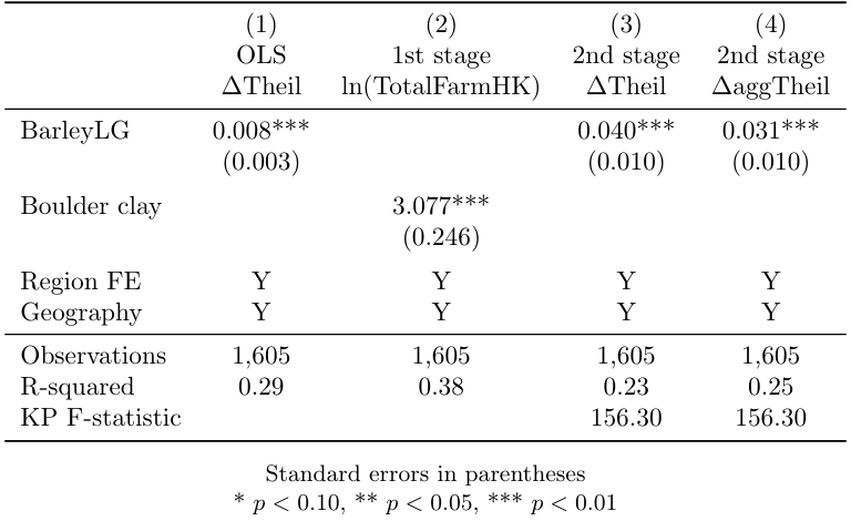
***Table A.4***

eststo clear

***Column (1) : OLS***
eststo ols1: qui reg D.Theil_c BygLG ln_area LnDistCPH Lat Long LnDistCoast i.region ///
  if year==1834, vce(robust)

eststo ols2: qui reg D.AggTheil_c BygLG ln_area LnDistCPH Lat Long LnDistCoast i.region ///
  i.year if year==1834, vce(robust)

***Column (2) : First-stage***
eststo fiv1: qui reg BygLG MLmean ln_area LnDistCPH Lat Long LnDistCoast i.region ///
  if year==1834 & ln_TotalFarmHK!=., vce(robust)

***Column (3) : Second-stage (diffTheil)***
eststo ivdiff1: qui ivregress 2sls D.Theil_c ln_area LnDistCPH Lat Long LnDistCoast ///
  i.region (BygLG = MLmean) if year==1834, vce(robust)
    estat firststage
    mat fstat = r(singleresults)
    estadd scalar Fstat = fstat[1,4]

***Column (4) : Second-stage (diffAggTheil)***
eststo ivdiff2: qui ivregress 2sls D.AggTheil_c ln_area LnDistCPH Lat Long LnDistCoast ///
  i.region (BygLG = MLmean) if year==1834, vce(robust)
    estat firststage
    mat fstat = r(singleresults)
    estadd scalar Fstat = fstat[1,4]

***Formation of Table A.4***
esttab ols1 fiv1 ivdiff1 ivdiff2, se star(* 0.10 ** 0.05 *** 0.01) b(3) r2 var(15) ///
  model(11) wrap keep(MLmean BygLG) mtitles("OLS" "first stage" ///
  "second stage (diffTheil)" "second stage (diffAggTheil)" ) stats(N r2 Fstat, ///
  labels("Observations" "R-squared" "KP F-statistic") fmt(%9.0fc 2 2)) ///
  indicate("Region FE = 2.region" "Geography = LnDistCPH" , labels(Y N)) label
Transitioning to another robustness test, presented in Table A.4 in the Appendix, we explore an alternative measure of land quality. In this test, rather than considering the total value of the parish’s HK, the authors focus solely on the amount of barley paid in tax as an indicator of land quality. This measure is derived from the digitization of a map presented by Frandsen in 1988. The results of this robustness check closely resemble the main estimations of table 1, underscoring the consistency and reliability of the analytical findings.
OLS regressions by replicating the columns 1 and 2 of Table A.4
***Table A.4***

eststo clear

***Column (1) : OLS***
eststo ols1: qui reg D.Theil_c BygLG ln_area LnDistCPH Lat Long LnDistCoast i.region ///
  if year==1834, vce(robust)

eststo ols2: qui reg D.AggTheil_c BygLG ln_area LnDistCPH Lat Long LnDistCoast i.region ///
  i.year if year==1834, vce(robust)

***Column (2) : First-stage***
eststo fiv1: qui reg BygLG MLmean ln_area LnDistCPH Lat Long LnDistCoast i.region ///
  if year==1834 & ln_TotalFarmHK!=., vce(robust)
In this analysis, we employ familiar Stata commands, akin to those
utilized in Table 1, with the only variable differing across each column
specification is the initial variable, corresponding to the dependent
variable: the change in the Theil index from 1682 to 1834 D.Theilc,
the change in the Theil index of 1834 aggregated to the size categories
of 1682 D.AggTheilc, and the amount of barley paid in tax as an
indicator of land quality BygLG, respectively. In line with our
approach of conducting the first-stage analysis, we introduce the
instrumental variable MLmean to the last regression equation. First,
the command eststo ols1 is used to store the estimation results, and
the results matrix is designated as ols1. The qui function,
signifying quietly, enables the temporary storage of results in the
matrix ols1 for the initial regression. Importantly, this function
ensures that the results of the regression are not displayed at this
point but are preserved under the name ols1 for subsequent
utilization. This approach proves particularly beneficial when authors
later aim to present a comprehensive table with multiple specifications.
Moreover, the reg function is utilized for Ordinary Least Squares
(OLS) estimation, running a regression with specified variables. In this
instance, the regression equation includes Theilc BygLG lnarea
LnDistCPH Lat Long LnDistCoast i.region. A conditional statement,
if year==1834 & lnTotalFarmHK!=., restricts the analysis to
observations where the year variable is equal to 1834, and
lnTotalFarmHK is not missing. This condition ensures a focused
examination of data relevant to the specified year and variable
condition. Furthermore, the use of the conditional if year==1834
filters the data, retaining only observations where the year
variable is equal to 1834. Lastly, the vce(robust) command is
incorporated to specify the use of robust standard errors. This
adjustment is made to account for potential heteroskedasticity and
correlation of errors, enhancing the reliability of the estimation
results.
IV regressions by replicating the columns 3 and 4 of the Table A.4
***Table A.4***

***Column (3) : Second-stage (diffTheil)***

eststo ivdiff1: qui ivregress 2sls D.Theil_c ln_area LnDistCPH Lat Long LnDistCoast ///
  i.region (BygLG = MLmean) if year==1834, vce(robust)
    estat firststage
    mat fstat = r(singleresults)
    estadd scalar Fstat = fstat[1,4]

***Column (4) : Second-stage (diffAggTheil)***
eststo ivdiff2: qui ivregress 2sls D.AggTheil_c ln_area LnDistCPH Lat Long LnDistCoast ///
  i.region (BygLG = MLmean) if year==1834, vce(robust)
    estat firststage
    mat fstat = r(singleresults)
    estadd scalar Fstat = fstat[1,4]
In this specific analysis, we focus on the second-stage of the
estimations with two dependent variables: D.Theilc, representing the
change in the Theil index from 1682 to 1834, D.AggTheilc,
representing the change in the Theil index of 1834 aggregated to the
size categories of 1682. The endogenous variable, the amount of barley
paid in tax as an indicator of land quality BygLG, is instrumented
by the share of boulder clay, utilizing MLmean as the instrumental
variable. This nuanced approach allows us to enhance the robustness of
the estimates and address potential biases in the endogenous variable.
In executing the second-stage of our analysis, employing the
eststo ivdiff1: qui command allows to store the estimation results
in a matrix named ivdiff1. This matrix captures the outcomes of the
two-stage instrumental variable regression facilitated by the
ivregress 2sls command. The regression equation includes explanatory
variables D.Theilc lnarea
LnDistCPH Lat Long LnDistCoast i.region, mirroring the structure of
OLS regressions.
Moreover, the specification (BygLG = MLmean) designates BygLG as
the endogenous variable, with MLmean serving as its instrumental
variable. An instrumentalization that is crucial to address potential
endogeneity concerns and fortifying the validity of the estimations. The
use of the conditional if year==1834 filters the data, retaining
only observations where the year variable is equal to 1834. To
account for heteroskedasticity and autocorrelation, the vce(robust)
command employs a robust variance-covariance matrix. Subsequently, we
encounter the lines of code that initially appeared daunting, but now,
through regular utilization, their functionality has become
comprehensible. Indeed, the estat firststage command is utilized to
display statistics from the first-stage of the IV regression, offering
insights into the validity of the instrumental variables. Further, the
mat fstat = r(singleresults) line stores the first-stage results in
a matrix named fstat, facilitating a comprehensive view of the
instrumental variable performance. Lastly, the
estadd scalar Fstat = fstat[1,4] command introduces a new scalar
variable Fstat into the main regression results. This step extracts
the F-statistic from the first-stage matrix fstat and assigns it to
Once again, for a more comprehensive understanding of the F-statistics
and its purpose, referring to the preceding Section 3.2.2 is
recommended. We would like to remind you that the results can be
independently observed directly using the same code without the qui
option, starting from reg or ivreg. This underscores the
flexibility of the code, allowing researchers to directly access and
analyze the regression outcomes without relying on the table generation
step.
Formatting Table A.4, an additional but optional step
***Table A.4***

***Formation of Table A.4***
esttab ols1 fiv1 ivdiff1 ivdiff2, se star(* 0.10 ** 0.05 *** 0.01) b(3) r2 var(15) ///
  model(11) wrap keep(MLmean BygLG) mtitles("OLS" "first stage" ///
  "second stage (diffTheil)" "second stage (diffAggTheil)" ) stats(N r2 Fstat, ///
  labels("Observations" "R-squared" "KP F-statistic") fmt(%9.0fc 2 2)) ///
  indicate("Region FE = 2.region" "Geography = LnDistCPH" , labels(Y N)) label
In the next step of our analysis, we construct a comprehensive table to
concisely present the findings from our prior regression analyses. It’s
important to emphasize that this stage isn’t isolated but rather
complements the groundwork laid in the preceding steps, where variables
were defined and regressions were conducted. The resultant table serves
as a visual tool to depict the relationships identified in our
regression models, thereby enhancing the clarity and communicative
impact of our analytical insights. In this stage, we use the esttab
command to generate a comprehensive table summarizing the results from
various models, including OLS, first-stage IV, and second-stage IV
regressions. The specified models, denoted as
ols1 fiv1 ivdiff1 ivdiff2, capture different aspects of the
regressions. The se star(* 0.10 ** 0.05 *** 0.01) option is employed
to display standard errors with significance stars, where asterisks
indicate different levels of significance with * for 0.10, ** for
0.05, and *** for 0.01. Setting b(3) limits, once again, the
number of decimal places for coefficient estimates to 3, contributing to
a cleaner presentation.
Including the R-squared r2 and limiting the number of decimals for
the R-squared to 15 digits var(15) provide additional insights into
the explanatory power of the models. Furthermore, the model(11)
option ensures that a maximum of 11 different models is displayed in the
table. To accommodate long variable names, the wrap command is
utilized, allowing for a more organized presentation. Moreover, the
keep(MLmean BygLG) option specifies the variables to be included in
the table, focusing on MLmean and BygLG. Model titles are
designated using the mtitles() option for clarity and organization.
Additional statistics, such as the number of observations (N),
R-squared, and the F-statistic, are included using the
stats(N r2 Fstat, labels("Observations" "R-squared" "KP F-statistic")fmt(%9.0fc 2 2))
option, providing a more comprehensive overview. Moreover, indicator
variables for fixed effects related to a specific region – here 2
representing Jutland – 2.region and geography LnDistCPH are
incorporated using the indicate() option. The labels(Y N))
allows to specify these fixed effects as Y if the fixed effects are
included or as N if they are not This offers further control in
understanding the impact of these factors on the results. Finally, the
label option ensures that variable labels are included in the table,
enhancing the interpretability of the presented information.
Once again, in the provided replication code by the authors, no specific
instruction regarding the exportation of tables has been included.
Therefore, we recommend users to add the command
using "NameOfYourTable.tex" right after the last variable mentioned
in esttab, just before the comma in front of se star, if they
intend to export the table in LaTeX format. Alternatively, users can use
the command using NameOfYourTable.txt", at the same location in the
code, if they prefer the table in a text format. This flexibility allows
users to choose the desired output format for the tables based on their
specific needs.
This last step to form a table can be employed in the context of other
studies to generate a clear and visually appealing table summarizing
regression results. However, it is crucial to emphasize that this step
is not indispensable for obtaining replication results. And although we
conducted a multitude of regressions in Section 3.5.1, it is noteworthy
that the final Table A.4 does not include the ols2 regression.
Finally, the results can be independently used directly with the same
code without the qui option, starting from reg or ivreg.
This highlights the flexibility of the code, allowing researchers to
directly access and analyze the regression outcomes without relying on
the table generation step. While the table contributes to a more
organized presentation, it is not a prerequisite for the replication
process, providing users with the option to tailor their analysis based
on specific preferences and requirements.
Our thorough replication process aimed to transparently convey each step of the analysis, ensuring clarity and reproducibility. We hope that our detailed descriptions provide a comprehensive understanding of the code and methodology employed. Moreover, we hope that this clarity enhances the accessibility of the article and facilitates further examination and validation by other researchers. We trust that transparency is crucial for fostering rigorous and collaborative research practices.
Authors: Auvray Adrien, Carette Anne-Laure, Tarlapan Alina, students in the Master program in Development Economics and Sustainable Development (2023-2024), Sorbonne School of Economics, Université Paris 1 Panthéon Sorbonne.
Date: December 2023